Type II Burst Analysis

Type II solar radio bursts are slowly drifting emission lanes produced by shock waves traveling outward through the corona. The plasma frequency falls with height, so the drift of the emission to lower frequencies traces the shock’s motion. The Type II tools fit the burst backbone and convert its frequency and drift into a shock height and speed using a coronal electron-density model.

The analysis chain

The analysis uses four tools, normally applied in this order:

Burst isolation restricts the data to the emission of interest (Section 8.2).
Maximum intensities extracts the frequency of peak emission in each time channel, or tracks the burst ridge (Sections 8.3 and 8.4).
Outlier removal discards points that do not belong to the burst (Section 8.5).
The Burst Analyzer fits the backbone and derives the drift rate, shock speed and shock height (Section 8.7).

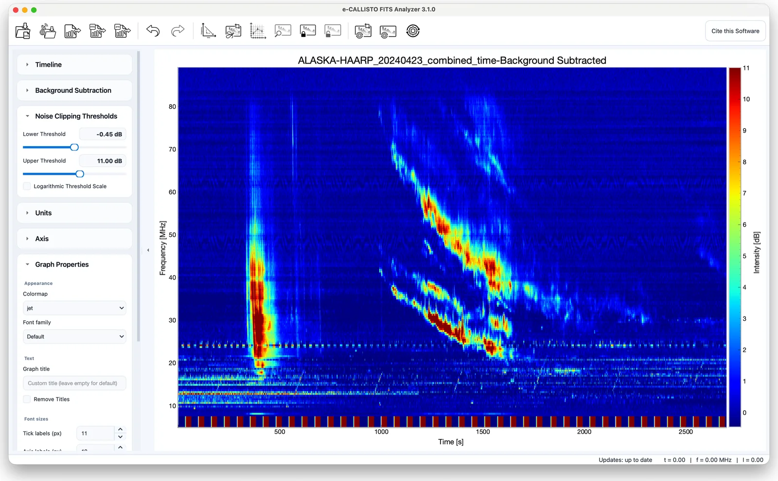
Each tool works on the spectrum as currently displayed: background-subtracted, RFI-cleaned or isolated. Figure 8.1 shows a background-subtracted spectrum containing a Type II burst.

**Figure 8.1.** A background-subtracted dynamic spectrum containing a Type II burst.

Burst isolation

The Isolate Burst toolbar tool (tool 9) draws a freehand lasso mask around the emission region of a burst. Background subtraction must be applied first.

Click Isolate Burst.
Press the mouse button, drag a loop around the burst, and release.

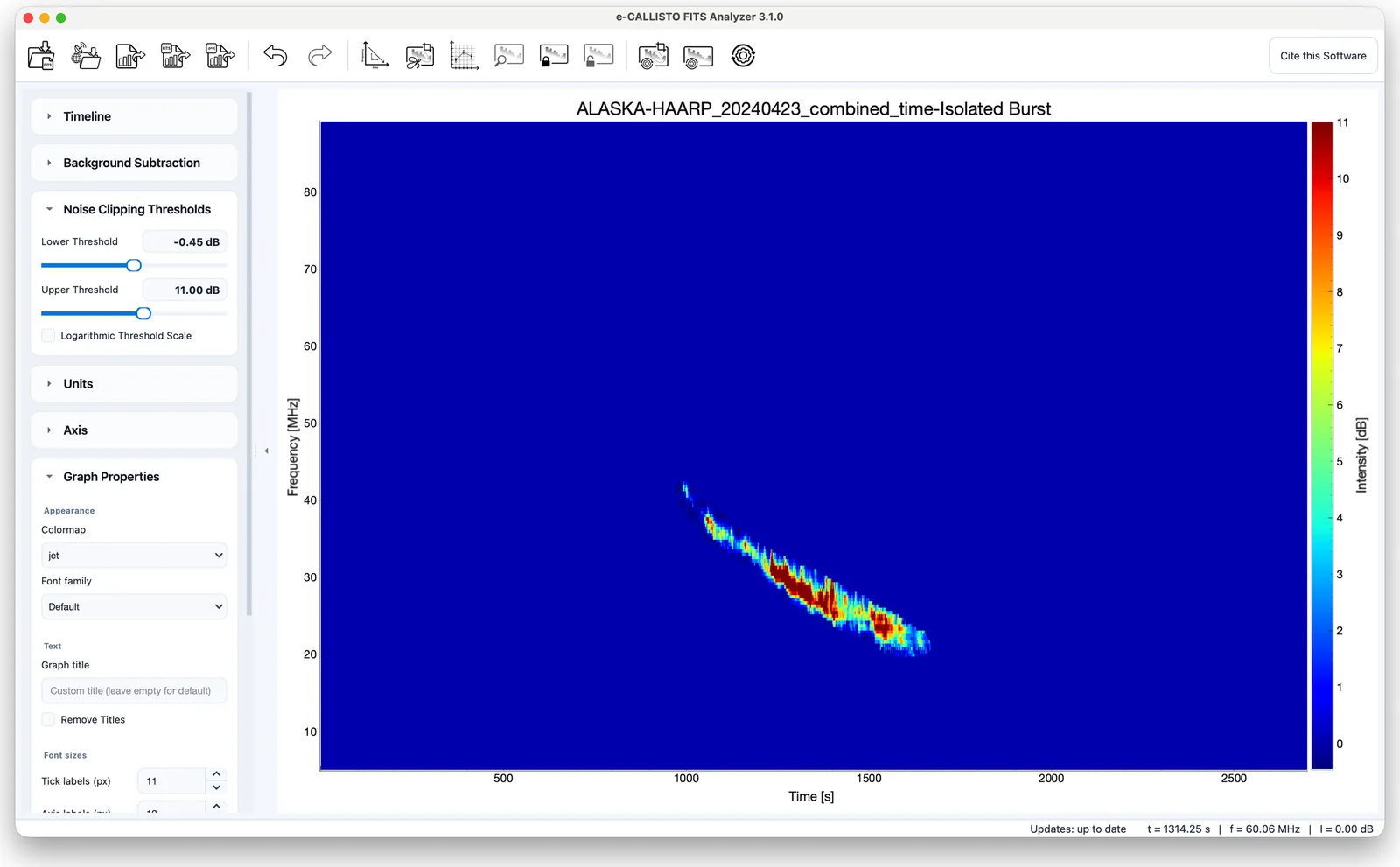
Only the data inside the loop are retained; everything outside is set to zero, which is the background level of the background-subtracted spectrum. This removes unrelated emission and residual noise from the analysis (Figure 8.2). Isolation can be undone with Ctrl+Z. The plot title changes to -Isolated Burst. The mask follows the drawn path on the displayed spectrum. Reset Selection (tool 14) clears the selection.

**Figure 8.2.** An isolated Type II burst lane.

The Maximum Intensities window

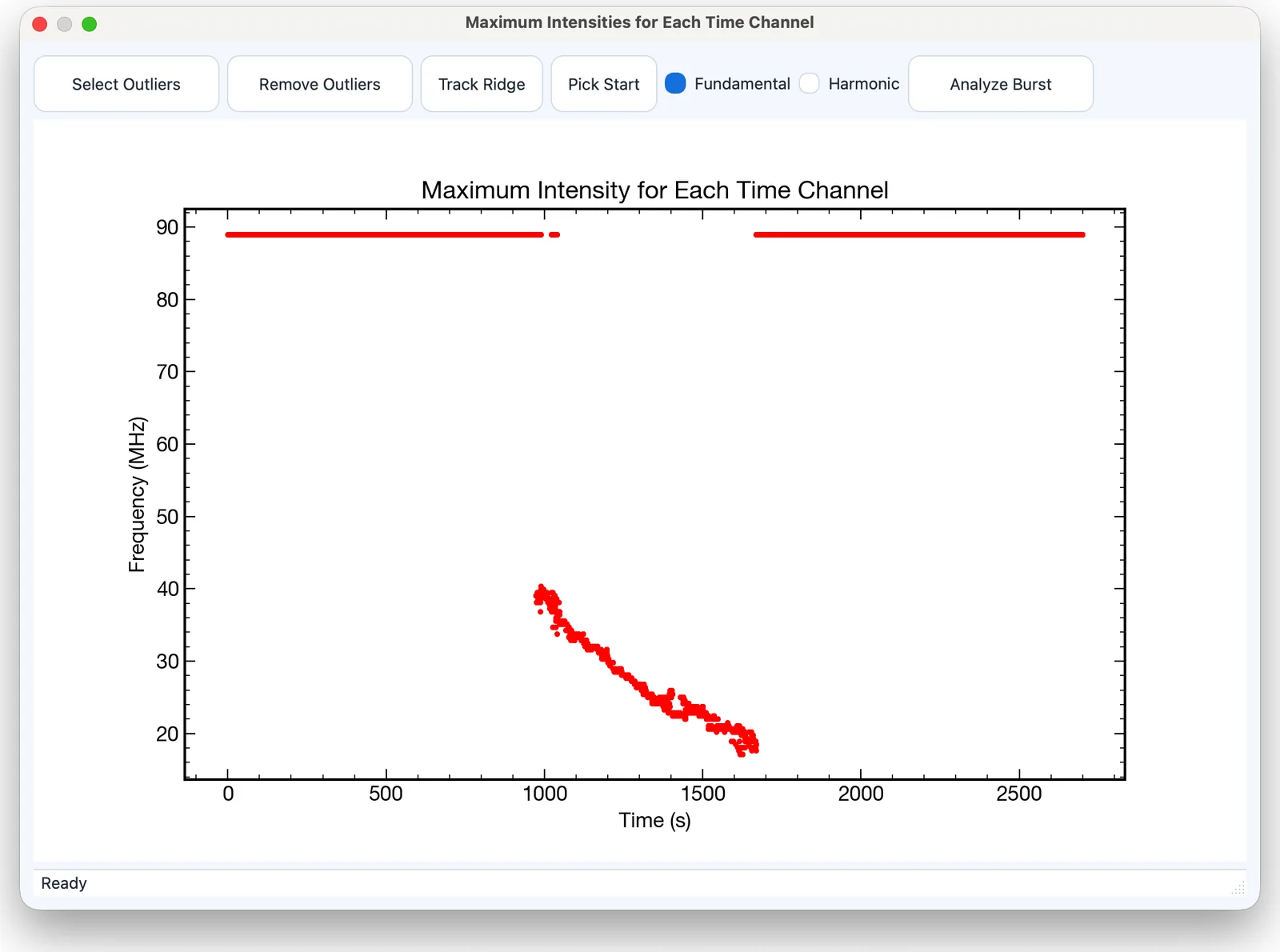
The Maximum Intensities window (Figure 8.3) shows, for each time channel of the displayed spectrum, the frequency at which the intensity is highest. These points trace the burst backbone that the Analyzer fits. Open it with the Plot Maximum Intensities toolbar tool (tool 10) or Analysis > Maximum Intensities > Open Maximum Intensities. When the maxima are taken from an isolated burst, time channels with no emission inside the mask are excluded.

Controls of the Maximum Intensities window.
Control	Function
Select Outliers	Draw a lasso around points to remove.
Remove Outliers	Remove the selected points.
Track Ridge	Replace the per-column maxima by an automatically tracked ridge (Section 8.4).
Pick Start	Click a point on the burst from which ridge tracking starts.
Fundamental / Harmonic	Whether the lane is fundamental or harmonic plasma emission (Section 8.6).
Analyze Burst	Open the Burst Analyzer with the current points.
File > Save As	Save the points as CSV: time channel, time (s) and frequency (MHz).
File > Export As	Save the plot as a figure (PNG, PDF, EPS, SVG, TIFF or JPG).
Edit > Reset All	Clear the selection, the ridge start point and the stored Analyzer state.
Edit > Restore Per-Column Maxima	Bring back the points replaced by ridge tracking.
Analyze > Open Analyzer	Open the Burst Analyzer.
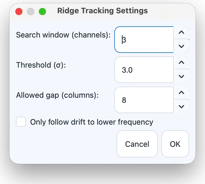
Analyze > Ridge Tracking Settings...	Parameters of the ridge tracker (Table 8.2).

The status bar at the bottom of the window reports the result of each action, for example the number of selected points.

Ridge tracking

Taking the brightest channel in every time column picks up RFI, a second burst or noise, leaving scattered points to remove by hand. Track Ridge follows the burst itself instead:

Tracking starts from the brightest point of the burst, or from a point chosen with Pick Start (marked with a star), and continues forwards and backwards in time, searching only a few channels around the ridge position in the previous column.
A channel that is bright for most of the file is treated as RFI and is not chosen as a starting point. An error is reported if a picked start point is not above the background.
Short dropouts in the burst are bridged. After a gap, tracking continues only once two consecutive columns show signal, so a single noise spike cannot extend the ridge. Tracking stops once the signal has stayed below the threshold for longer than the allowed gap.
Each peak is refined to sub-channel frequency.

The tracked points replace the per-column maxima; outlier removal, the fundamental/harmonic choice and Analyze Burst work on them as before. Edit > Restore Per-Column Maxima brings the original points back.

Ridge Tracking Settings.
Setting	Description	Default
Search window (channels)	Maximum movement of the ridge between two consecutive time columns (1–100).	3
Threshold ( $\sigma$ )	Minimum height of a peak above the background, in robust standard deviations (0–50).	3.0
Allowed gap (columns)	Number of consecutive columns below the threshold before tracking stops (0–1000).	8
Only follow drift to lower frequency	Restricts the ridge to move toward lower frequencies with time, as in Type II and Type III bursts.	Off

The Ridge Tracking Settings dialog. — **Figure 8.4.** The **Ridge Tracking Settings** dialog.

Outlier removal

Outliers are removed manually in the Maximum Intensities window:

Click Select Outliers and draw a lasso around the unwanted points (Figure 8.5).
Click Remove Outliers.

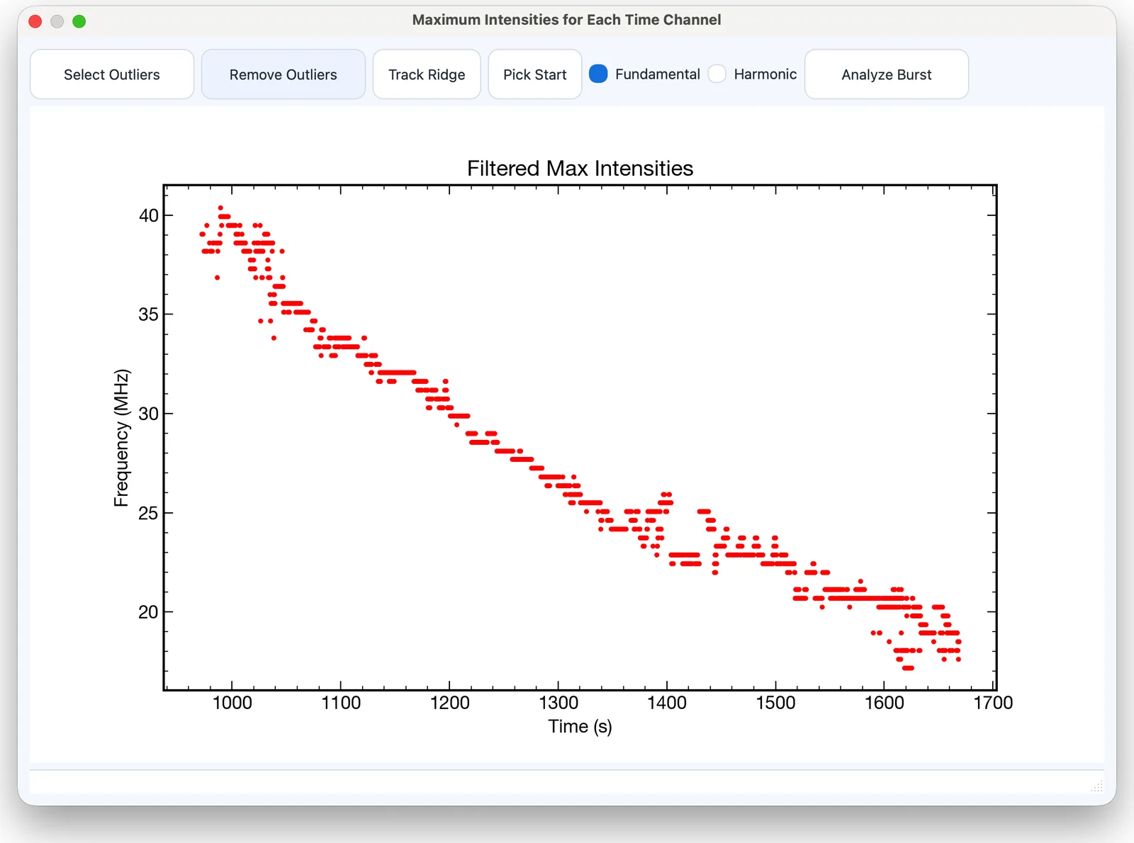
**Figure 8.5.** Selecting outliers with the lasso in the Maximum Intensities window.

When Processing > Maximum Intensity > Auto-Clean Isolated Burst Outliers is ticked (the default), outliers are also removed automatically whenever the maxima are taken from an isolated burst. The manual tools remain available in either case.

Fundamental and harmonic emission

Type II emission occurs at the local plasma frequency (fundamental) and at twice that frequency (harmonic). Select Harmonic when the fitted lane is the harmonic. The observed frequencies and drift rates are then divided by two before the shock parameters are calculated, so that heights and speeds always refer to the plasma frequency. Saved summaries keep both the converted values and the observed reference values.

The Burst Analyzer

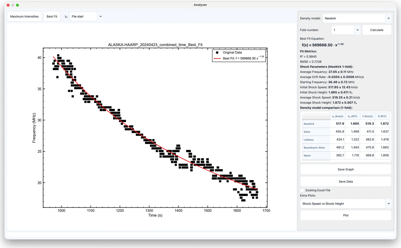
The Burst Analyzer (Figure 8.6) fits the burst backbone with a power law and derives the frequency drift rate, shock speed and shock height, with the goodness of fit. Open it with Analyze Burst or Analyze > Open Analyzer in the Maximum Intensities window.

Controls and displays of the Burst Analyzer.
Control or display	Function
Maximum Intensities	Plot the extracted points.
Best Fit	Fit the points with a power law and plot the fit.
t₀	Time origin of the power law (Section 8.7.1).
Density model	Coronal density model for heights and speeds (Section 8.7.3).
Fold-number	Multiplier 1–4 applied to the model density; press Calculate after changing it.
Best Fit Equation	The fitted power law.
Fit Metrics	$R^2$ and RMSE of the fit.
Shock Parameters	Derived quantities with uncertainties (Table 8.4).
Density model comparison	Initial and average shock speed and height from all five models (Section 8.7.4).
Save Graph	Save the plot on show as a figure.
Save Data	Save the results to an Excel workbook (Section 8.7.6).
Existing Excel File	Append to an existing workbook instead of creating a new one.
Extra Plots and Plot	Additional plots (Section 8.7.5).

Power-law fit and the time origin

The backbone is fitted as $\begin{equation} f(t) = a\,(t - t_0)^{-b}, \label{eq:power-law} \end{equation}$ where $f$ is the frequency in MHz, $t$ the time in seconds, and $a$ and $b$ the fitted parameters. The drift rate at each point follows from the derivative, $\mathrm{d}f/\mathrm{d}t = -ab\,(t-t_0)^{-b-1}$ . On the Best Fit graph the points are drawn as filled black squares and the fitted power law as a red curve, with a boxed legend.

Because a power law depends on where $t=0$ lies, the fitted exponent, drift rate and shock parameters depend on the chosen time origin. $t_0$ is selected from the t₀ list next to Best Fit:

File start: measures time from the start of the loaded data (the default).
Burst onset: places $t_0$ one time sample before the first fitted point, so that every point lies on the curve.
Custom time: uses a time that you enter, in UT when the start time of the file is known and otherwise in seconds from the start of the file.

Changing $t_0$ re-runs the fit automatically. The graph keeps the data’s own time axis, and the equation shows $(x - t_0)$ whenever $t_0$ is not the file start.

Shock parameters

Table 8.4 defines the quantities in the Shock Parameters block. The heading names the density model and fold in use, for example Shock Parameters (Newkirk 1-fold).

Shock parameters reported by the Burst Analyzer.
Quantity	Definition
Average Frequency	Mean frequency of the maximum-intensity points (MHz), with its standard error.
Average Drift Rate	Mean of the fitted drift rate along the backbone (MHz/s).
Starting Frequency	The 90th percentile of the fitted frequencies, taken as the start of the burst (MHz).
Initial Shock Speed	Shock speed at the starting frequency (km/s).
Initial Shock Height	Heliocentric height at the starting frequency ( $R_\odot$ ).
Average Shock Speed	Mean shock speed along the backbone (km/s), with its standard error.
Average Shock Height	Mean height along the backbone ( $R_\odot$ ), with its standard error.

Background: from drift rate to shock speed

The emission frequency is identified with the local plasma frequency, $f_p \approx 8.98\times10^{-3}\sqrt{n_e}$ MHz for an electron density $n_e$ in cm $^{-3}$ . A density model $n_e(r)$ therefore maps each frequency to a heliocentric height $r$ , and the drift rate to a radial speed, $\begin{equation*} v = \left|\frac{\mathrm{d}f}{\mathrm{d}t}\right| \left|\frac{\mathrm{d}r}{\mathrm{d}f}\right|, \qquad \frac{\mathrm{d}r}{\mathrm{d}f} = \frac{2\,n_e}{f\,|\mathrm{d}n_e/\mathrm{d}r|}. \end{equation*}$ Uncertainties are propagated linearly from the drift-rate and frequency errors. The results are only as good as the density model, which describes an average corona and can differ from the actual medium by large factors; the fold number scales the model density to account for denser structures such as streamers.

Density models

Shock heights and speeds are calculated from one of five coronal electron-density models (Table 8.5). Changing the model recalculates the shock parameters immediately. The fold number (1–4) multiplies the model density; press Calculate after changing it. The formulas are given in Appendix D.

Coronal electron-density models.
Model	Reference
Newkirk (default)	Newkirk (1961)
Saito	Saito et al. (1977)
Leblanc	Leblanc et al. (1998)
Baumbach–Allen	Baumbach (1937); Allen (1947)
Mann	Mann et al. (1999)

Models other than Newkirk are evaluated between the photosphere ( $1\,R_\odot$ ) and 1 AU. A frequency that a model cannot reach in this range — for example above about 116 MHz for the 1-fold Saito model — has no height, and is shown as a dash rather than an extrapolated value.

Density-model comparison

The Density model comparison table below the shock parameters lists the initial shock speed $v_0$ , initial height $h_0$ , average speed $\bar v$ and average height $\bar h$ obtained with every model at the current fold, with the selected model in bold. It shows at a glance how strongly the derived kinematics depend on the assumed corona.

Additional plots

Choose an entry in Extra Plots and click Plot to show: Shock Speed vs Shock Height, Shock Speed vs Frequency or Shock Height vs Frequency. These plots use the selected density model.

Saving graphs and data

Save Graph writes whichever plot is on show — maximum intensities, best fit or an additional plot — as an OriginPro-style graph on a white page in PNG, PDF, EPS, SVG, TIFF or JPG format.

Save Data writes one row of results to an Excel workbook (.xlsx). With Existing Excel File ticked, you choose a workbook and the row is appended, which builds an event table over many analyses. The columns are listed in Table 8.6.

Columns of the Burst Analyzer Excel export.
No.	Column
1–2	Observation date; station
3–5	Best-fit equation; $R^2$ ; RMSE
6–9	Average frequency and error; average drift rate and error
10–11	Starting frequency and error
12–15	Initial shock speed and error; initial shock height and error
16–19	Average shock speed and error; average shock height and error
20	Absolute value of the average drift rate
21	Density model
22	$t_0$ in seconds from the start of the file

The density model and $t_0$ are also saved in projects and named in project reports. Projects saved before these options existed open with the Newkirk model and the file start as $t_0$ , matching how they were calculated.