The Solar Image Analysis Window

Solar Image Analysis is a multi-mission imaging workspace for extreme-ultraviolet (EUV) disk images, magnetograms, coronagraph images and heliospheric images. It retrieves image sequences from the solar archives or reads local FITS files, displays and processes them, measures eruptions and their kinematics, and models the coronal magnetic field. Open it with Analysis > Solar Image Analysis in the main window.

This chapter describes the window, its menus and sessions, and how image data are obtained. Display and processing are described in Chapter 17, measurements in Chapter 18 and magnetic-field modeling in Chapter 19.

Supported observables

Table 16.1 lists the observables that can be retrieved. Local FITS files from these and other solar instruments can be loaded as well.

Observables available in Solar Image Analysis.
Instrument	Class	Observables
SDO/AIA (Lemen et al. 2012)	EUV/UV disk	94, 131, 171, 193, 211, 304, 335, 1600 and 1700 Å
SDO/HMI (Scherrer et al. 2012)	Magnetograph	Magnetogram, Continuum (Intensitygram), Dopplergram; vector field (Section 17.10)
SOHO/EIT	EUV disk	171, 195, 284 and 304 Å
SOHO/LASCO (Brueckner et al. 1995)	Coronagraph	C2, C3
STEREO-A/B SECCHI (Howard et al. 2008)	EUV disk, coronagraph, heliospheric imager	EUVI 171, 195, 284 and 304 Å; COR1, COR2; HI1, HI2
GOES/SUVI	EUV disk	94, 131, 171, 195, 284 and 304 Å

The sidebar shows only the tool groups that apply to the instrument class of the loaded data (or, before loading, of the selected observable); see Table 16.4.

Window layout

The window is divided into the regions numbered in Figure 16.1 and described in Table 16.2.

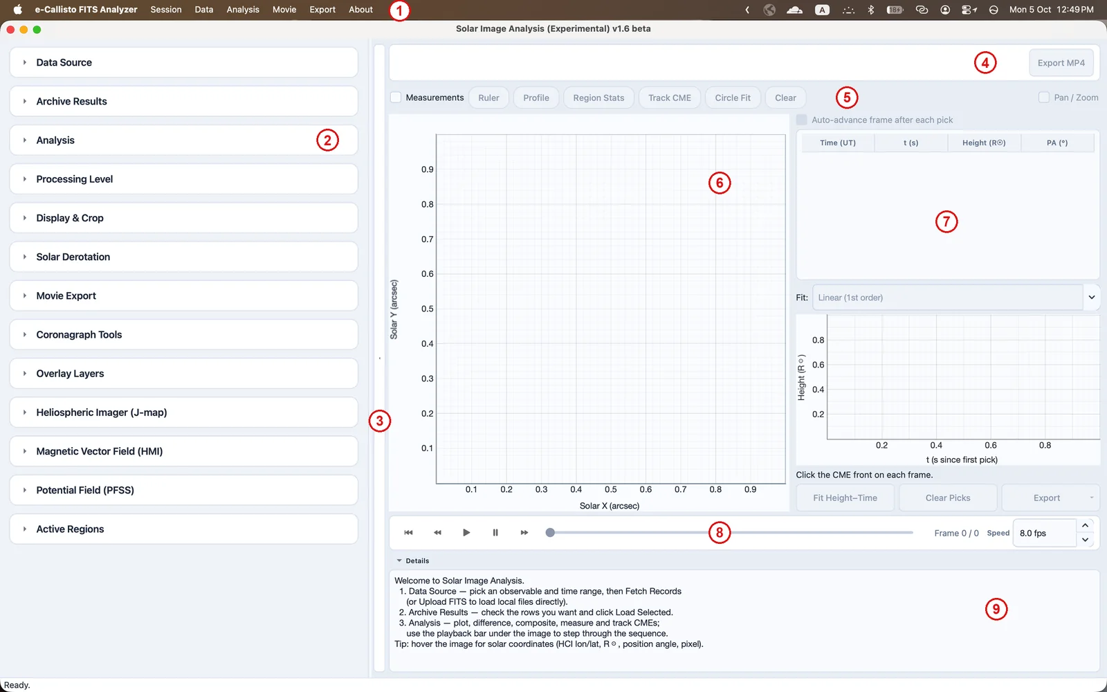
**Figure 16.1.** The Solar Image Analysis window with its regions numbered.

Regions of the Solar Image Analysis window.
No.	Region	Description
1	Menu bar	Session, Data, Analysis, Movie, Export and About (Section 16.2.1).
2	Sidebar	Collapsible cards that read from top to bottom as the workflow: get data, choose records, analyze, then display, export and instrument-specific tools.
3	Sidebar handle	Hides or shows the sidebar.
4	Header bar	Live cursor readout — distance from Sun center in $R_\odot$ , position angle, heliographic coordinates on the disk, and pixel — and the one-click Export MP4 button.
5	Measure toolbar	The Measurements switch, the Ruler, Profile, Region Stats, Track CME, Circle Fit and Clear tools, and Pan / Zoom (Chapter 18).
6	Image canvas	The current frame, titled with instrument, wavelength and time.
7	CME tracking panel	Measurement table, live height–time graph and kinematic fit; active when Measurements is ticked (Section 18.4).
8	Playback bar	Rewind, previous, play, pause and next buttons, the frame scrubber, the frame counter (Frame n / N) and the Speed in frames per second.
9	Details drawer	Results and warnings of every operation. Click Details to collapse it; drag the divider above it to resize.

The playback speed set in the playback bar is used for playback and for exported movies. While a sequence plays, or while a contrast slider is dragged, the canvas switches to a fast preview that subsamples the display; full resolution returns as soon as playback stops. Measurements, statistics and exports always use the full-resolution data.

Menus

Menus of the Solar Image Analysis window.
Command	Function
Session > Open Session…	Open an `.ecsolar` session (Section 16.4).
Session > Save Session / Save Session As…	Save the session (`Ctrl+S` / `Ctrl+Shift+S`).
Data > Fetch Archive Records	Search the archive (Fetch Records).
Data > Find Latest Available	Find the newest available data (Find Latest).
Data > SOHO Live Preview (Helioviewer)	Near-real-time SOHO quicklook images (Section 16.3.3).
Data > Load Selected (to cache)	Download and load the ticked records.
Data > Save Selected to Disk…	Download the ticked records to a folder.
Data > Upload FITS Files	Load local FITS files.
Data > Use Analyzer Window	Copy the time range of the main window’s spectrum.
Data > Stop Download/Search	Cancel the running operation.
Data > Reset All (clear cache & defaults)	Clear the cache and restore default settings.
Analysis > Plot Frames, Running Difference, Composite	Display modes (Section 17.1).
Analysis > Identify Active Regions, Fetch NOAA/HEK Labels	Active-region tools (Section 17.5).
Analysis > Compare Viewpoint…	Compare with a second observer (Section 17.6).
Analysis > GCS CME Fitting…	Open GCS fitting at the time of the displayed frame (Chapter 20).
Analysis > Reset Loaded Frames	Restore the frames as loaded.
Movie > Rewind, Back, Play, Pause, Forward	Playback.
Movie > Build Movie	Export a movie (Section 17.11).
Export > Export Plot, Export Cropped FITS, Export Regions CSV, Export MP4	Exports (Section 17.11).
About > About Solar Image Analysis…	Version information.

Table 16.4 lists the sidebar cards in order, and the instrument classes for which each is shown.

Sidebar cards of Solar Image Analysis.
Card	Shown for	See
Data Source	all	Section 16.3.1
Archive Results	all	Section 16.3.2
Analysis	all (disk tools for disk imagers and magnetographs only)	Section 17.1
Processing Level	AIA and SUVI	Section 16.3.4
Display & Crop	all	Section 17.2
Solar Derotation	all	Section 17.3
Movie Export	all	Section 17.11
Coronagraph Tools	coronagraphs	Section 17.7
Overlay Layers	coronagraphs	Section 17.8
Heliospheric Imager (J-map)	HI1, HI2	Section 17.9
Magnetic Vector Field (HMI)	HMI	Section 17.10
Potential Field (PFSS)	disk imagers, magnetographs, synoptic maps	Chapter 19
Active Regions	disk imagers, magnetographs	Section 17.5

Obtaining image data

The Data Source card

The Data Source card (Figure 16.2) defines what to retrieve and how.

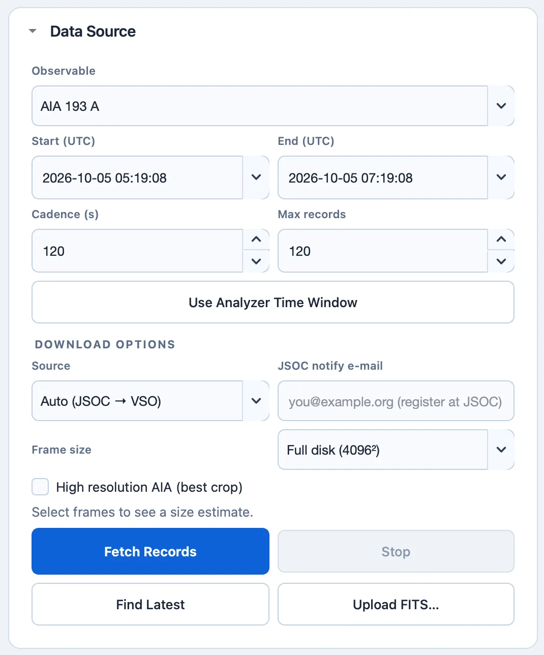
Observable: the instrument and wavelength or product (Table 16.1).
Start (UTC), End (UTC): the time range.
Cadence (s): the sampling interval between frames (0–3600 s; default 120 s).
Max records: the maximum number of records to list (1–5000; default 120).
Use Analyzer Time Window: copies the start and end times of the spectrum in the main window, so that the images match the radio burst being studied.

Download options (SDO)

Source: Auto (JSOC → VSO) tries the Joint Science Operations Center (JSOC) first and falls back to the Virtual Solar Observatory (VSO); JSOC (fast) returns direct, compressed AIA files and is usually much faster; VSO (classic) uses the VSO only.
JSOC notify e-mail: JSOC requires a one-time, free registration of an e-mail address at https://jsoc.stanford.edu/ajax/register_email.html. The address is remembered.
Frame size: Full disk (4096²), Binned ½ (2048²), Binned ¼ (1024²) or Cutout (region). Binned and cutout frames are produced by JSOC, so only the reduced data are transferred; they require the JSOC source and e-mail. For a cutout, enter the Centre X″, Centre Y″, Width″ and Height″ in arcseconds from disk center.
High resolution AIA (best crop): requests full-resolution AIA products. Files are larger, but cropped views keep more detail.

An estimate of the download size is shown below the options when records are selected.

Actions

Fetch Records: searches the archive; the matching records appear in Archive Results. Stop cancels a running search or download; files already completed remain in the cache.
Find Latest: scans the archive backwards to find the newest data actually available for the observable. This is useful for SOHO/LASCO, whose calibrated archive can lag real time by many months, and may take a minute or two.
Upload FITS…: loads solar FITS files from disk without an archive search.
Live Preview (Helioviewer): shown for SOHO/LASCO and SOHO/EIT (Section 16.3.3).

The Archive Results card

The Archive Results table lists the records found, with the columns Use, Start UTC, Source, Size and File ID. Tick records in the Use column, or use Select All and Deselect All, then:

Load Selected downloads the ticked records into the working cache and loads them for analysis; or
Save to Disk… downloads them to a folder you choose, for keeping.

The Analysis card then summarizes what is loaded (instrument, number of frames and configuration).

SOHO data

The archive serves two files for every SOHO/EIT observation, the calibrated Level 1 file and the raw level-zero file. The window chooses one per observation: Level 1 where it exists and the raw file otherwise. Level 1 processing runs about a year behind the raw archive, so recent searches return raw frames and older ones calibrated frames; a window that straddles the boundary loads as two configuration groups. The calibrated SOHO/LASCO archive also lags real time. For a date beyond the newest archived data, the search falls back to the nearest available data and says so. Use Live Preview to see the most recent SOHO images.

Live Preview (Helioviewer)

Live Preview (Helioviewer) opens the SOHO/… Near-Real-Time Preview (Helioviewer) window (Figure 16.3) with the newest quicklook image of SOHO/LASCO C2 or C3 or SOHO/EIT, usually updated within about an hour. These browse images are for situational awareness, not for analysis.

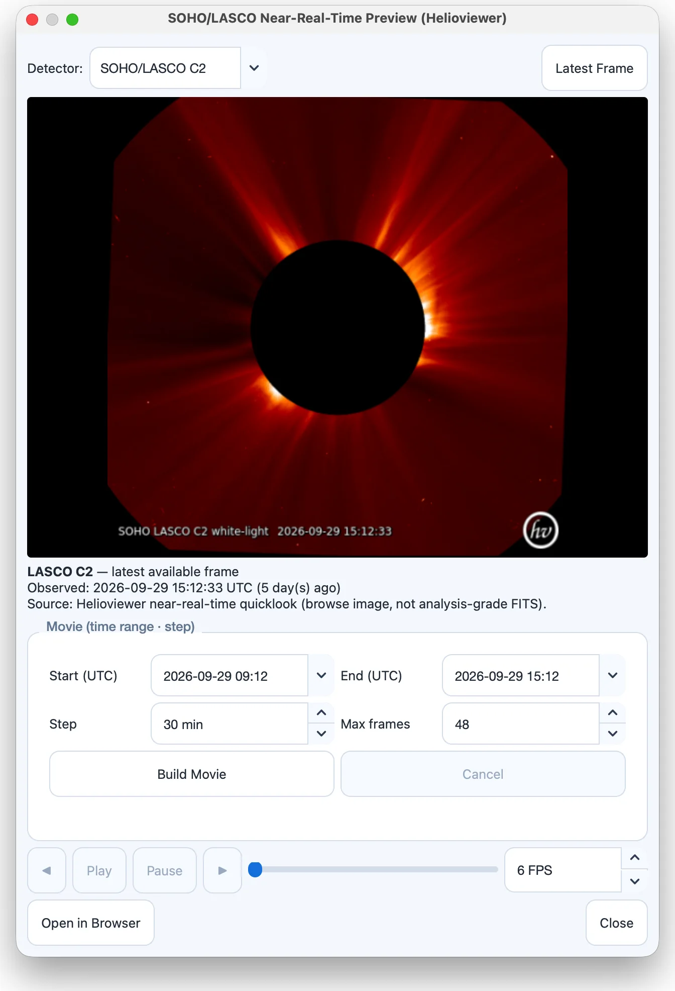
Passband / Detector, Latest Frame: choose the EIT passband or LASCO detector, and reload the newest image.
Movie (time range · step): set Start (UTC), End (UTC), Step (minutes) and Max frames, then Build Movie to fetch one frame per step and play them with ◀, Play, Pause, ▶ and an FPS setting. Cancel stops the fetch. The frame cap protects the Helioviewer service.
Open in Browser: opens the view on the Helioviewer web site.

Processing level

Downloads always fetch the archive’s base product. For instruments that publish more than one processing level, the Processing Level card selects the level that is displayed and analyzed:

SDO/AIA: Level 1 (as downloaded), the archive product; or Level 1.5 (registered here), computed locally with aiapy (Barnes et al. 2020), which applies the master pointing, rotates the image to solar north, rescales it to 0.6 arcsec per pixel and centers the Sun.
GOES/SUVI: Level 1b (as downloaded), single calibrated exposures; or Level 2 (archive composite), NOAA’s high-dynamic-range composites, which are downloaded separately when selected.

Apply Level re-derives the loaded sequence at the selected level; any crop or derotation is re-applied afterwards. The status line reports the level in use. The card is hidden for instruments that offer only one level.

Sessions

A Solar Image Analysis session (.ecsolar) is a single file that reopens an analysis exactly where it was left. It embeds the original FITS frames, so it survives a cleared cache or a move to another computer (at the cost of a large file), together with the data source, the display, crop and playback state, the CME measurements (height–time picks, circle fits and fit order) and the PFSS settings. The PFSS solution itself is not stored; one click on Compute PFSS reproduces it. Sessions are opened and saved from the Session menu (Ctrl+S, Ctrl+Shift+S).