
Coronal Magnetic Field Modeling (PFSS)
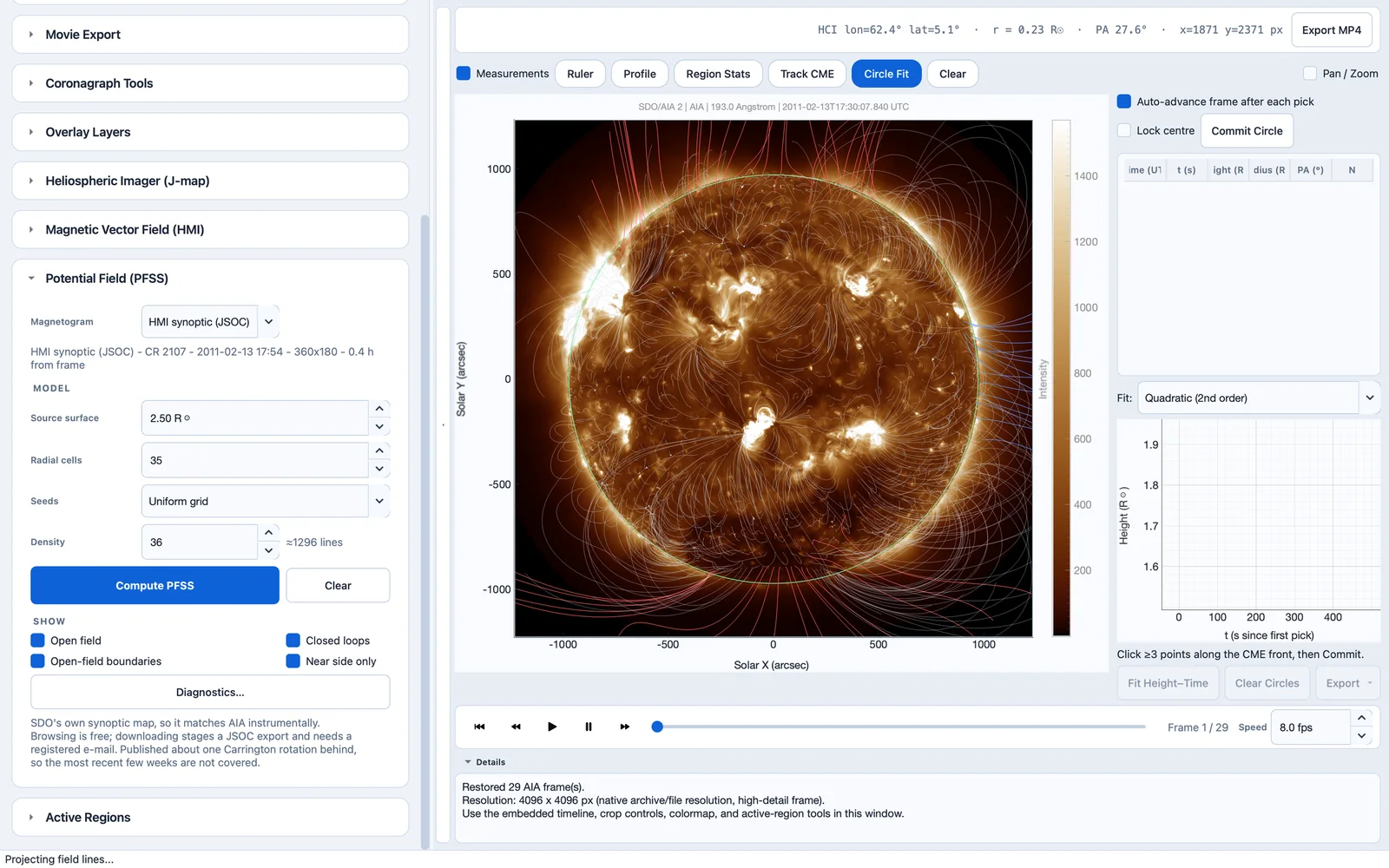
An EUV image shows where the coronal plasma is, not where the magnetic field is. The Potential Field (PFSS) card of Solar Image Analysis extrapolates the coronal magnetic field from a photospheric magnetogram with the potential-field source-surface model (Schatten et al. 1969; Altschuler and Newkirk 1969) and draws the resulting field lines over the disk (Figure 19.1), so that the modeled loop topology and coronal holes can be compared with the image. The card is shown for disk imagers, magnetographs and synoptic maps.
Background: the PFSS model
The model assumes a current-free (potential) field between the photosphere and a spherical source surface a few solar radii out, where the field is forced to be radial to mimic the solar wind dragging it open. Field lines that reach the source surface are open and feed the solar wind; the others are closed loops. The open-field footpoint regions are the model’s coronal holes, and the polarity-inversion line on the source surface marks where the heliospheric current sheet leaves the model.
Caution
AIA images carry no magnetic-field information, so the boundary condition comes from a synoptic magnetogram — a full-Sun map assembled from central-meridian observations over a whole solar rotation. The model therefore describes the global field around your observation, never the instantaneous field, and the far side is always at least two weeks old. The card shows how far the map’s date is from the displayed frame; that offset is the number to judge the result by.
Settings
| Setting | Description |
|---|---|
| Magnetogram | The boundary condition (Section 19.1.1). For GONG ADAPT, Realization (0–11) chooses one of the twelve flux-transport realizations; for Local FITS file..., Browse… selects the file. The line below names the loaded map and its time offset from the frame. |
| Source surface | Height at which the field is forced radial (1.5–10 ; default 2.5 ). Lowering it opens more field. |
| Radial cells | Radial grid resolution between the photosphere and the source surface (10–150; default 35). More is smoother and slower. |
| Seeds | Where field lines start (Section 19.1.2). |
| Density | Seed density (4–64; default 12, about 150 field lines). It controls both speed and legibility; the hint beside it estimates the number of lines. |
Magnetograms
- GONG synoptic
-
the ground-based GONG synoptic map (Harvey et al. 1996), updated daily and available for any date from 2006 on. No registration is needed; this is the usual choice.
- HMI synoptic (JSOC)
-
SDO’s own synoptic map, instrumentally consistent with AIA. Searching is free, but downloading stages a JSOC export and needs the registered e-mail set in the Data Source card. The series is published about one Carrington rotation behind, so the most recent weeks are not covered.
- GONG ADAPT
-
maps from the ADAPT flux-transport model, which estimates the unobserved far side instead of leaving it weeks old and usually improves open-field predictions. One file holds twelve realizations, which differ mostly on the far side.
- Local FITS file...
-
a synoptic map you already have. It must be a full-Sun Carrington map; plate-carrée maps are reprojected to equal-area automatically.
Downloaded magnetograms are cached, so changing a model parameter and solving again does not download the map again. Unmeasured pixels, such as the polar gaps in GONG maps, are filled with zero so that the solution can be computed; their number is reported.
Seeds
- Uniform grid
-
an equal-area sample over the visible hemisphere.
- Open-field regions
-
a coarse survey is traced first, and then lines are started only where the field is open. This shows coronal-hole connectivity without closed loops dominating the picture.
- Current crop
-
concentrates the lines inside the crop rectangle.
- Clicked points
-
traces one line from each point clicked on the disk. This needs the PyQtGraph renderer.
Tracing costs about 1.6 ms per field line, so a solution takes a few seconds at most, but beyond about 150 lines the field lines start to hide the image they are compared with. Prefer Open-field regions to a high density when coronal-hole connectivity is what you want.
Computing and displaying the model
Compute PFSS downloads the magnetogram if needed, solves the potential field and traces the field lines in the background; Clear removes the overlay and the solution. The Show options toggle the layers without recomputing:
- Open field
-
lines reaching the source surface, colored by the sign of the radial field at their footpoint: red outward, blue inward.
- Closed loops
-
lines returning to the photosphere, drawn in gray.
- Open-field boundaries
-
outlines of the open-field footpoint regions, for comparison with the dark coronal holes in 193 or 211 Å images.
- Near side only
-
(on by default) hides lines rooted on the far hemisphere. Such lines are not hidden behind the disk once they rise above the limb, so they would otherwise be drawn as arcs outside the disk with no visible footpoint. Clear it for the geometrically complete picture.
Stepping through a sequence re-projects the same solution onto each frame instead of solving again. This is correct, because the synoptic map is valid across the rotation while the observer’s view changes from frame to frame.
Diagnostics
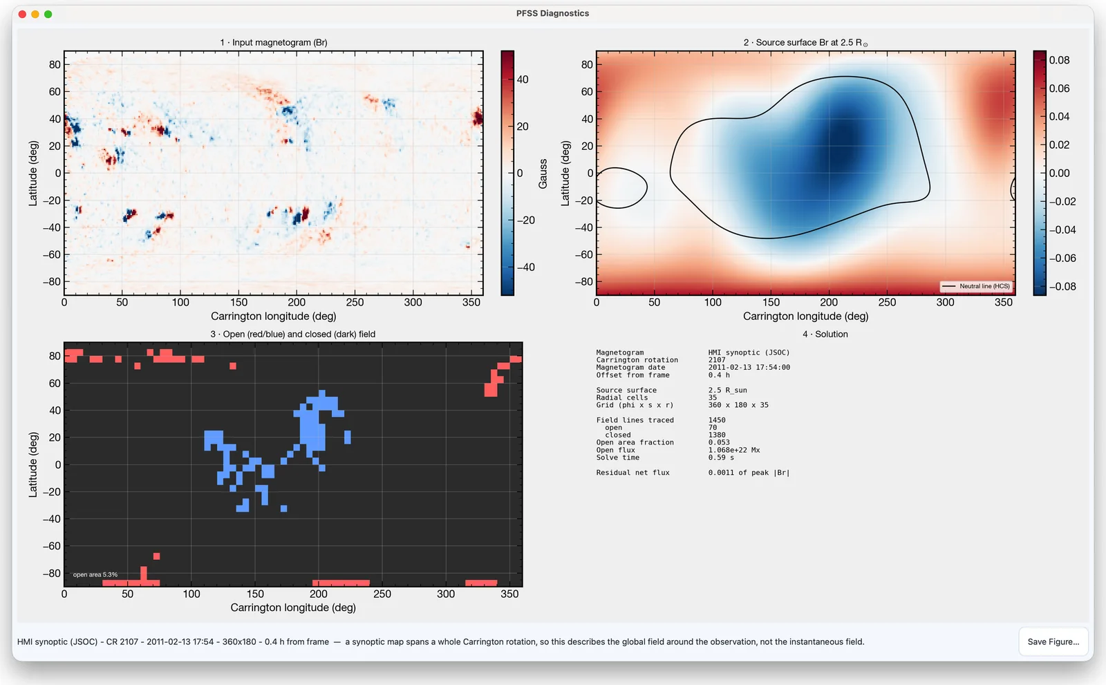
Diagnostics… opens a four-panel window that documents the solution (Figure 19.2):
the input magnetogram () with its provenance;
the radial field at the source surface with its neutral line, where the heliospheric current sheet leaves the model — the model’s most directly testable prediction;
the open (red and blue) and closed (dark) footpoint map in Carrington projection;
the solution statistics, including the open flux, the open-area fraction and the number of filled pixels.
Save Figure… saves all four panels as one image (PNG, PDF or SVG).
Note
PFSS modeling uses the sunkit-magex package (Stansby et al. 2020), which is included
in the installers. When the application is run from source without it,
the card remains visible but disabled and shows the command to install
it. Sessions store the PFSS settings, not the solution (Section 16.4).