
A spectrum that changes with time
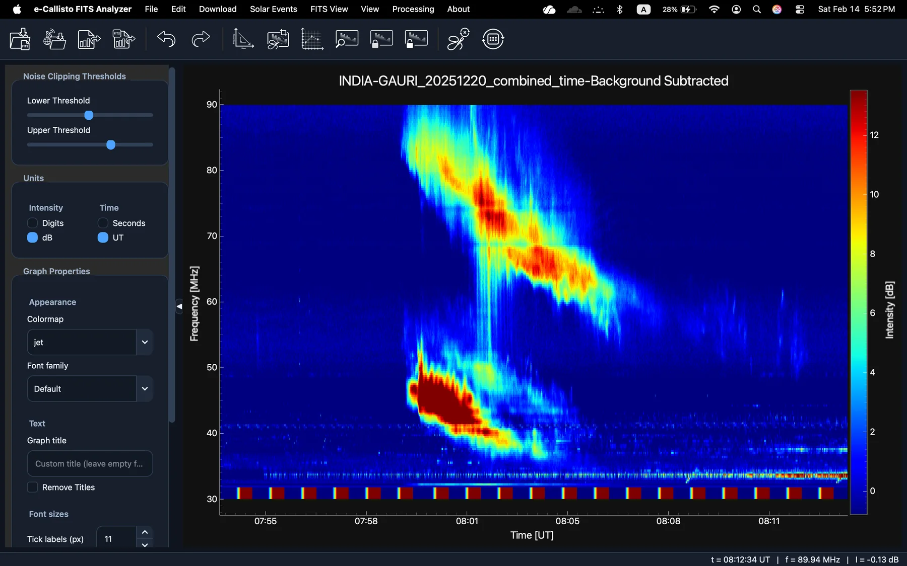
A dynamic spectrum displays radio intensity as a function of time and frequency. In a CALLISTO observation, time runs along the horizontal axis, frequency along the vertical axis, and colour represents intensity. The instrument’s native frequency range is 45–870 MHz; an individual observation’s coverage depends on station configuration and any converters.
The e-CALLISTO network brings together distributed solar radio spectrometers around the world. Its observations support research, education and radio-frequency interference monitoring. Explore the e-CALLISTO network.
From plasma to radio emission
Solar radio bursts can carry signatures of energetic electrons and shocks. Under a plasma-emission interpretation, radiation occurs near the local electron plasma frequency or its harmonic. The plasma frequency is approximately:
fp [kHz] ≈ 8.98 √(ne [cm⁻³])The emission mode matters: assigning the same observed frequency to fundamental or harmonic emission produces different inferred electron densities. A spectrum alone does not always resolve that ambiguity. Background: NASA-hosted solar radio emission overview (§5.1.3).
Frequency drift and the corona
A drifting emission lane traces a change in observed frequency over time. Converting that drift to a radial height or speed requires an emission assumption and a coronal electron-density model. Version 3.1.0 provides the Newkirk, Saito, Leblanc, Baumbach–Allen and Mann models with 1–4 fold multipliers, and compares the resulting shock speeds and heights side by side.
For a chosen monotonic density model, a frequency can be mapped to a model height. The resulting height–time curve gives a model-dependent speed. Compare plausible models and document the frequency range, time origin and fitting choices. The formulas used by the analyzer are collected in Appendix D of the user guide.
Imaging and CME geometry
Coronagraph images show a CME projected onto the plane of the sky, so a leading-edge height measured in one view is a projected height. Fitting a Graduated Cylindrical Shell to images from several viewpoints, such as STEREO and SOHO, constrains a three-dimensional model of the flux rope and gives deprojected heights within that model. A Potential Field Source Surface extrapolation adds the global magnetic context around the event.
Keep measurement and interpretation distinct
- Radio-frequency interference can resemble or obscure solar features. Inspect raw data and compare independent stations.
- Thresholds change display contrast; they do not establish detection significance.
- Shock and magnetic-field estimates rely on physical assumptions, emission-lane identification and the selected model.
- GCS reconstruction depends on viewing geometry, front identification and image timing. Small residuals do not establish accuracy.
- PFSS models use synoptic magnetograms assembled over a full solar rotation, so they describe the global field rather than the instantaneous one.