
From images to measurements.
Explore SDO, SOHO and STEREO data, track an eruption and connect it with the magnetic structure of the Sun.
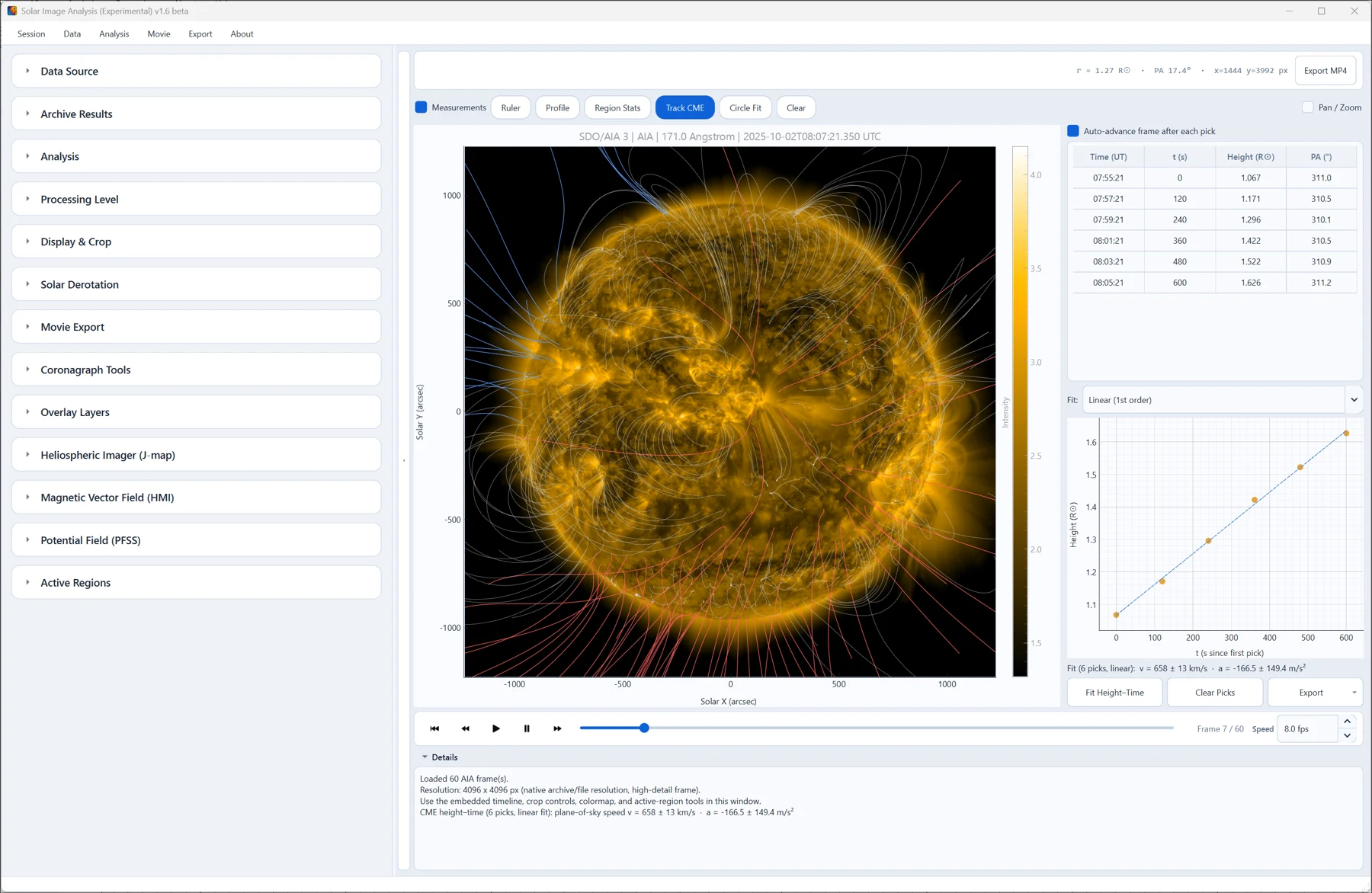
A connected imaging workflow
Open Analysis → Solar Image Analysis in the desktop analyzer. Search instrument archives or load local FITS images. Available sources include SDO/AIA and HMI, SOHO/EIT and LASCO, and STEREO/SECCHI EUVI, COR1, COR2 and HI.
- Load and inspect. Select an instrument and time range, then browse the frame sequence. Adjust the display, crop a region and compare running or base differences.
- Measure the event. Use a ruler, intensity profile or region statistics. In Track CME mode, select the same leading-edge feature in successive frames to build a height–time table.
- Fit the evolution. Compare linear, quadratic or cubic fits and their covariance-based uncertainties. Check the selected feature and frame times before interpreting the result.
- Save your work. Export measurements as CSV, create figures and GIF/MP4 movies, or save an
.ecsolarsession to retain your measurements and fitting state.
See an exported image sequence
Magnetic context with PFSS
New in v3.1.0, the Potential Field Source Surface workflow extrapolates the coronal field from a GONG, HMI, GONG ADAPT or local synoptic magnetogram. Overlay open and closed field lines and coronal-hole boundaries on the AIA disk, and inspect the input map, source-surface field and neutral line under Diagnostics…. Solves run in the background and downloads are cached.
Synoptic maps represent global magnetic context assembled over time. PFSS is a model of that field, and a visual overlay should be interpreted with its assumptions and observation times in mind.
Image layers and CME geometry
Reproject compatible layers, adjust opacity and build contextual composites, now including SOHO/EIT 171, 195, 284 and 304 Å. Leading-edge tracking gives projected heights; Circle Fit models the CME as an expanding sphere resting on the solar surface (h = 1 R☉ + 2r). For a shared three-dimensional model across coronagraph viewpoints, continue to GCS fitting.
Every window and option is described in Part V of the user guide.