Opening and Combining Data
This chapter describes the file types the main window reads, the ways of opening them, and the rules and options for combining several files into one dynamic spectrum.
Supported files
The main window reads CALLISTO dynamic spectra in FITS format, compressed or uncompressed:
uncompressed files:
.fit,.fits;gzip-compressed files:
.fit.gz,.fits.gz.
Upper-case suffixes such as .FITS are accepted.
Combination relies on the standard CALLISTO file name,
STATION_YYYYMMDD_HHMMSS_FC, from which the station, start
time and focus code are read. Files converted from the Learmonth
spectrograph (Section 13.1) follow the same
conventions.
ARTEMIS-IV files
FITS files from the ARTEMIS-IV radio spectrograph (Thermopylae,
Greece) in its ARTLOOK format are recognized automatically.
On loading:
the hours-based UT time axis is converted to the internal time axis;
intensities are labeled and scaled as ADC counts, with the instrument’s conversion of 58.51 counts per dB used for the dB scale; and
the observation opens background subtracted, because the receiver’s channel gains span more than an order of magnitude.
Opening files
Use any of the following:
File > Open, the Open / Load toolbar tool, or
Ctrl+O;drag the files onto the main window;
File > Recent Files (Section 5.2.1);
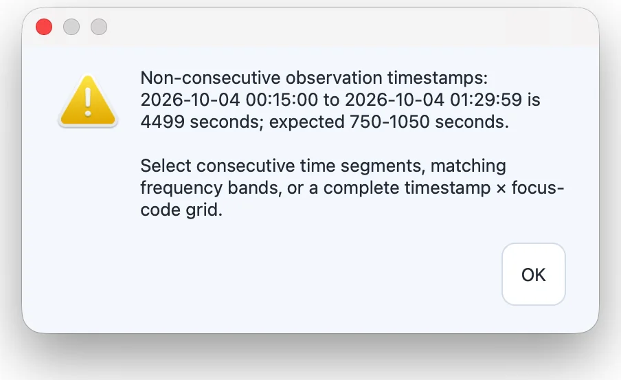
When one file is selected, it is displayed at once. When several files are selected, the application determines whether they can be combined in time, in frequency, or in both (Section 5.3) and, if so, combines them into a single spectrum. If the selection cannot be combined, a message explains why (Figure 5.1). If the current work has unsaved project changes, you are asked whether to save them first.
After loading, the analysis controls and the Graph Properties panel become active, and the sidebar’s Timeline panel lists the observations that make up the dataset.
Recent files
File > Recent Files lists the last ten FITS selections. A combined set is a single entry, combined again when reopened; hovering over an entry shows its files. An entry whose files have been moved or deleted is removed from the list with a message. Clear Recent Files empties the list.
Combining files
CALLISTO observations are fragmented in time (15-minute files) and often in frequency (several receivers or focus codes). The application can merge them along either axis or both. The rules are summarized in Table 5.1.
| Combination | Requirements |
|---|---|
| Time | Same station and focus code; consecutive observations whose start times are 750–1050 s apart (normally 15 minutes). Sequences may continue across UTC midnight. |
| Frequency | Same station, date and observation start time; distinct focus codes; identical time axes. Bands may be separated by a gap or may overlap (Section 5.3.1). |
| Time frequency | A complete grid of at least two consecutive timestamps and at least two focus codes, with the same set of focus codes at every timestamp. |
A selection that contains extra files is searched for a combinable subset; for example, selecting a whole day of files together with one stray file still finds the grid within it. All files of one combined dataset must come from the same station.
For a time frequency grid, the bands are first combined at each timestamp with one shared gap and overlap policy; the application checks that every result has the same frequency grid, and then joins the results in time order. Incomplete grids, duplicate timestamp and focus-code pairs, non-consecutive timestamps and incompatible axes are rejected with a detailed message.
Combined datasets keep their provenance: exported FITS files,
projects and reports record the original list of source files and the
combination method (time, frequency or
time_frequency).
Frequency gaps and overlaps
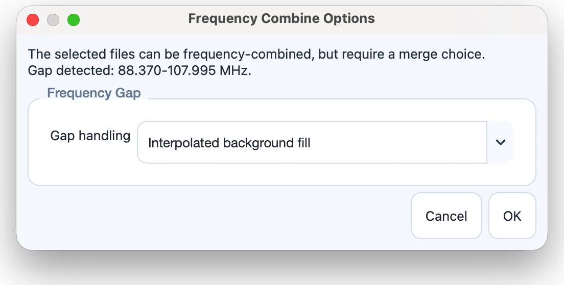
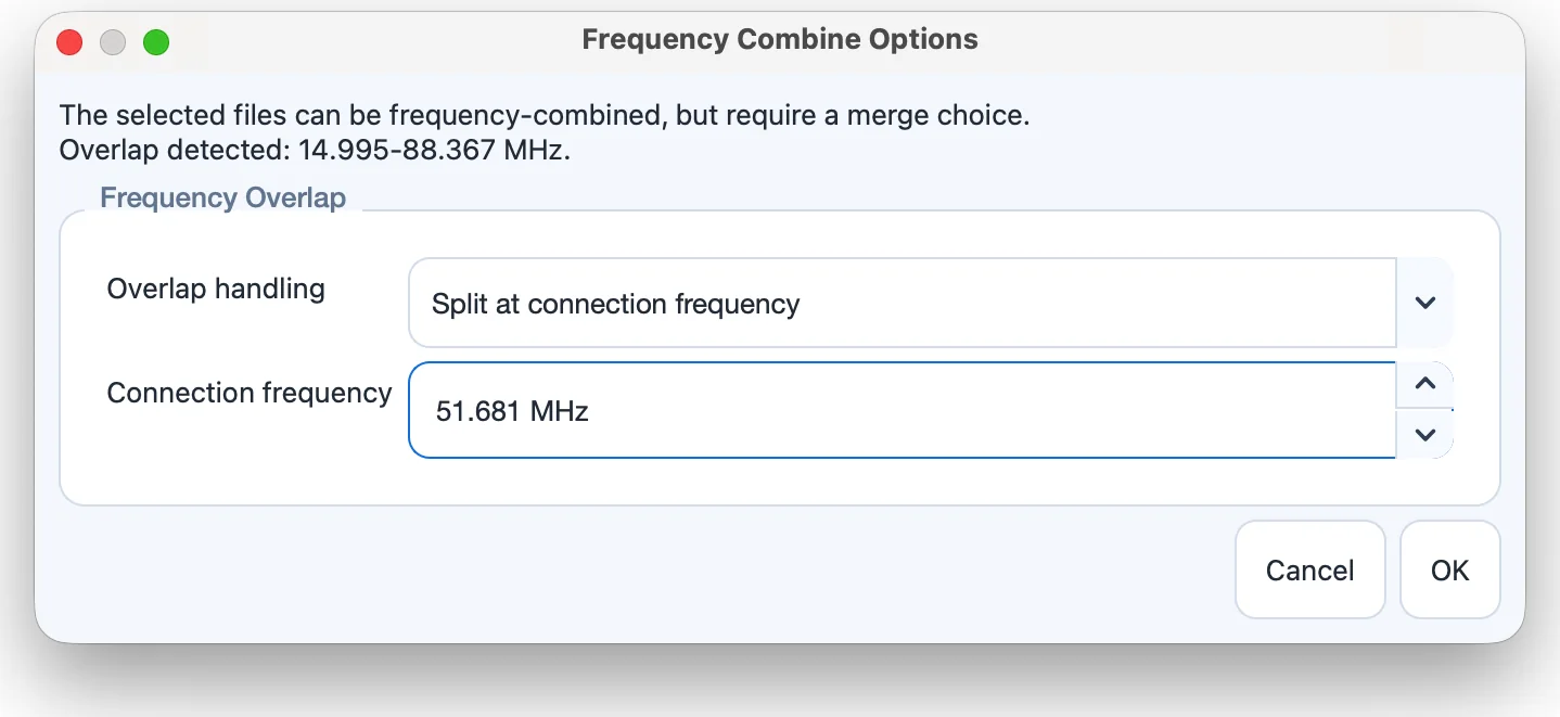
When the selected bands leave a gap between them, or overlap, the Frequency Combine Options dialog asks how to handle it before the combined spectrum is imported (Figures 5.2 and 5.3). The detected gap or overlap range is shown at the top of the dialog. The chosen option is stored in the metadata of the combined dataset.
- Interpolated background fill
-
fills the gap with background values interpolated between the edges of the two bands.
- Gray-hatched blank gap
-
leaves the gap without data and displays it as a gray-hatched region, so that it is clearly distinguished from observed data.
- Average edge background fill
-
fills the gap with the average background level of the band edges on either side.
- Zero fill
-
fills the gap with zeros.
- Split at connection frequency
-
uses the lower band below the Connection frequency and the higher band above it. The connection frequency is proposed automatically and can be edited.
- Use lower-frequency file
-
keeps the data of the lower-frequency file in the overlapping region. The file name is shown in the option when there is a single overlap.
- Use higher-frequency file
-
keeps the data of the higher-frequency file in the overlapping region.
- Reject overlap
-
cancels the combination.
The Combine FITS Files dialog
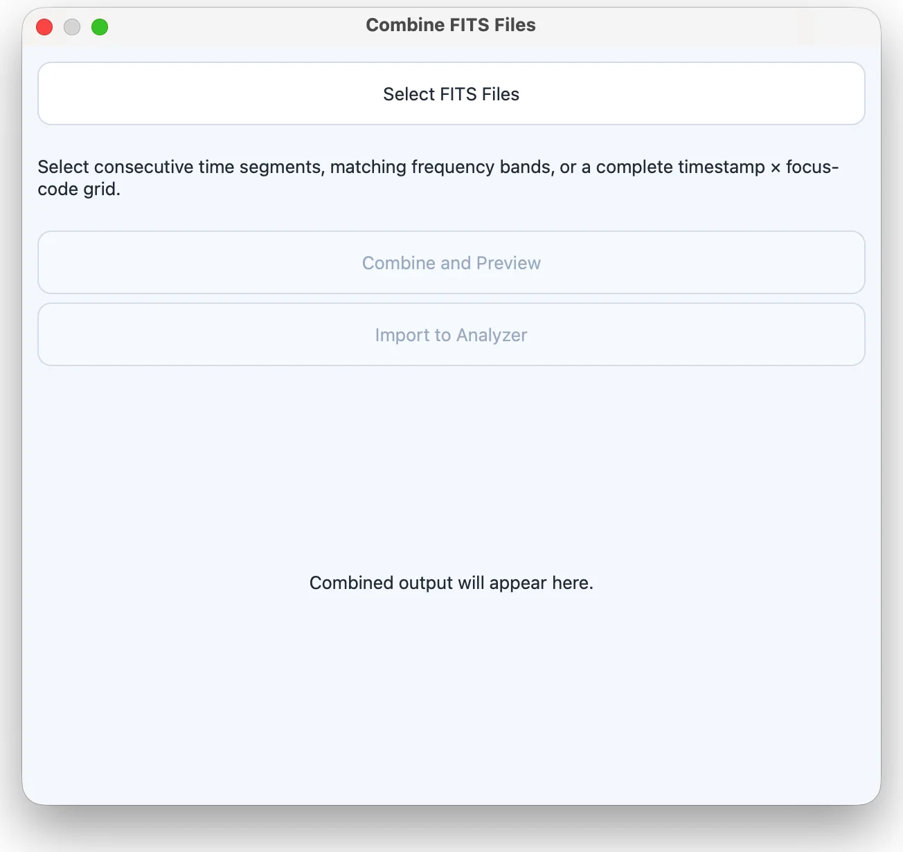
File > Combine FITS Files... opens a dialog for selecting, validating and previewing a combination before it is imported (Figure 5.4).
Click Select FITS Files and choose the files. The dialog inspects them and reports whether they form a valid time, frequency or time frequency combination.
For a frequency combination, choose the gap and overlap handling and, if needed, the connection frequency in the Frequency Combine Options group. In this dialog the overlap choices are labeled Keep low band in overlap and Keep high band in overlap.
Click Combine and Preview to see the combined spectrum in the dialog.
Click Import to Analyzer to load the result into the main window.
Viewing the FITS header
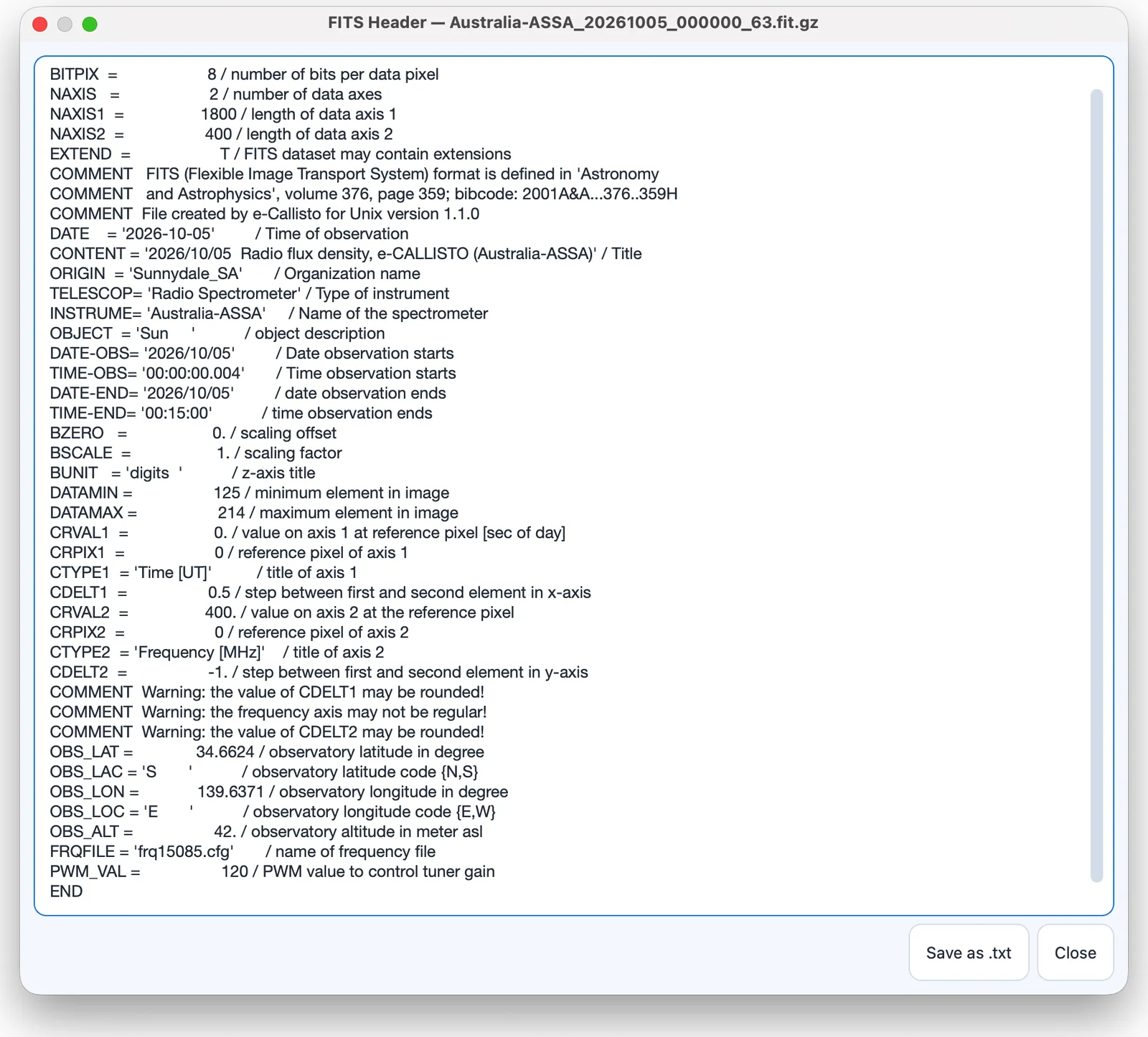
View > View FITS Header shows the primary header of the loaded file (Figure 5.5). Save as .txt writes the header to a text file.