Measurements and CME Kinematics

The Measure toolbar above the image provides click-driven tools for distances, intensity profiles, region statistics and CME tracking. The CME tracking panel to the right of the image collects the measurements of a sequence and fits their kinematics.

Enabling the tools

Tick Measurements in the Measure toolbar to enable the tools; the CME tracking panel becomes available at the same time. One tool is active at a time. A right-click or Esc cancels a pick in progress without leaving the tool. Results are shown in the status line and appended to the Details drawer. Pan / Zoom, at the right of the toolbar, enables dragging and scroll-wheel zooming of the image; the zoom is kept while the movie plays, and unticking it returns to the full frame.

Tools of the Measure toolbar.
Tool	What it does
Ruler	Two clicks give the plane-of-sky distance in arcseconds, $R_\odot$ and Mm, and the position angle (measured from north toward east).
Profile	Two clicks plot the intensity along the cut, for example across a loop, a filament or a CME front, in the Intensity Profile window.
Region Stats	Summarizes the crop rectangle: pixel count, mean, median, minimum, maximum, standard deviation and intensity-weighted centroid (arcsec). Enable Rectangle crop first to choose the region.
Track CME	One click per frame on the leading edge of a CME. The height is its distance from disk center. Best for limb events.
Circle Fit	Three or more clicks along a circular front per frame. Best for eruptions near disk center.
Clear	Resets every measurement: picks, circles, table and overlays.

The 3-D reconstruction of CMEs from several viewpoints is performed in the separate GCS CME Fitting window (Part VI), opened from Analysis > GCS CME Fitting….

Tracking a CME

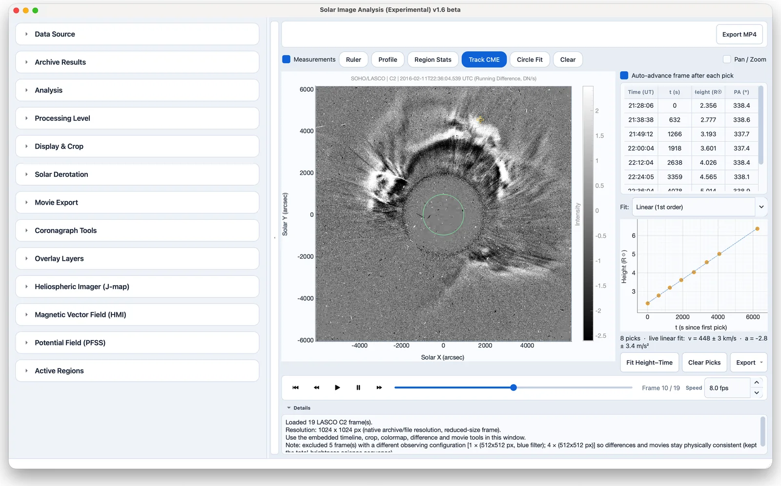
Track CME measures a height–time profile with one click per frame (Figure 18.1).

Go to the first frame in which the CME front is visible.
Select Track CME and click the leading edge. The pick is added to the tracking table and, with Auto-advance frame after each pick ticked (the default), the next frame is shown.
Repeat on each frame, then choose the fit order and click Fit Height–Time.

The height is the plane-of-sky distance of the clicked point from Sun center in $R_\odot$ ; the position angle (PA) is recorded with it. The tool works on any imager — EUVI, AIA, SUVI, COR, LASCO and HI. Clicking again on a frame replaces its pick.

**Figure 18.1.** CME tracking with the height–time graph in the tracking panel.

Fitting a circle to a CME front

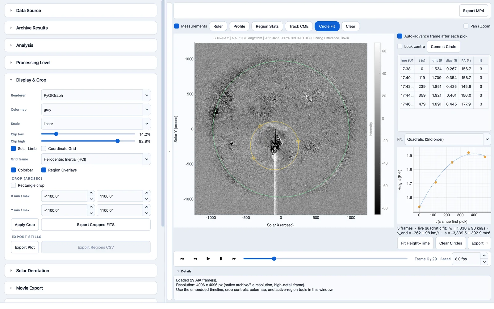
For eruptions near disk center the front expands as a growing dome rather than moving outwards from the limb, and a single leading-edge click has no well-defined origin. Circle Fit models the CME as a uniformly expanding sphere resting on the solar surface (Figure 18.2).

Select Circle Fit and click three or more points along the visible front. The least-squares circle is drawn from the third click and tightens with each further point.
Click Commit Circle (Ctrl+Return). The frame’s result is added to the table and the next frame is shown.
Repeat on each frame, then click Fit Height–Time.

Each row gives the height $h = 1\,R_\odot + 2r$ , where $r$ is the fitted radius (the sphere’s top is one diameter above the surface), the radius in $R_\odot$ , the position angle of the center and the number of points. The fit residual, the center and the leading-edge distance from disk center appear in the row’s tooltip. Re-committing a frame replaces its entry.

Click a wide arc. A short arc is fitted, but it constrains the radius very weakly, and the panel warns when the arc spans less than about 30°.
Lock centre freezes the center at its current fitted value so that later frames fit the radius alone. Use it once the dome has stopped drifting.

The fit uses Taubin’s method (Taubin 1991), which is not biased toward small radii on partial arcs, and works in helioprojective arcseconds so that the front remains a circle when the plate scale differs between the axes.

**Figure 18.2.** Circle fitting of an on-disk CME front.

The CME tracking panel

The tracking panel shows the measurements of the active tool:

Table: for Track CME: Time (UT), t (s) since the first pick, Height (R☉) and PA (°); for Circle Fit: additionally Radius (R☉) and the number of points N.
Height–time graph: the measured heights against time, with the live fit.
Fit: the polynomial order: Linear, Quadratic or Cubic. Changing it refits the points already in the graph.
Fit Height–Time: fits the points and reports the speed and acceleration below the graph.
Clear Picks / Clear Circles: removes the measurements of the active tool.
Export: Table as CSV…, or Graph (PNG, PDF, EPS, SVG, TIFF, JPG)… drawn in light mode and the OriginPro style.

Background: height–time fits

Linear: $h = h_0 + v t$ : one plane-of-sky speed for the whole track. The acceleration is taken from a companion quadratic fit, as in the CDAW CME catalog.
Quadratic: $h = h_0 + v_0 t + \tfrac12 a t^2$ : constant acceleration, with the speed reported at the first and last frame.
Cubic: adds a constant jerk, with the speed and acceleration reported at both ends.

Every value carries a $1\sigma$ uncertainty propagated from the fit covariance, so the correlations between the polynomial terms are included. A fit of degree $n$ needs $n+1$ points, and $n+2$ before an uncertainty can be estimated; with fewer points the value is shown without an error rather than with a misleading zero. Heights from Track CME are plane-of-sky distances, so the derived speeds generally underestimate the true radial speed; Circle Fit heights rely on the assumption of a sphere expanding from the surface.

The measurements — picks, circles, the lock state and the fit order — are saved in .ecsolar sessions (Section 16.4).