The Sidebar Panels
The sidebar on the left of the main window groups the controls used most often while working on a spectrum. It contains eight sections, from top to bottom: Timeline, Background Subtraction, Noise Clipping Thresholds, Units, Axis, Graph Properties, Analysis Summary and Ruler Measurement. Each section is a card with a clickable header that collapses or expands it; the state of every card is remembered between sessions. The whole sidebar can be hidden with the arrow handle on the left edge of the plot.
Timeline
A loaded dataset knows which station, focus codes and observation times it came from. The Timeline panel (Figure 6.1) lists them and extends or trims the dataset in place, without returning to the downloader.
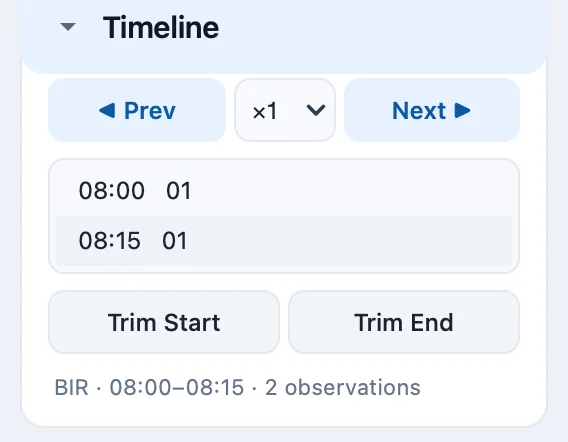
- ◀ Prev / Next ▶
-
Fetch the observation before the first, or after the last, and time-combine it into the spectrum (
Ctrl+Shift+LeftandCtrl+Shift+Right, also in the Edit menu). - Step selector (1, 2, 4, 8)
-
The number of observations added per click.
- Observation list
-
One row per observation, giving its start time and focus code(s).
- Trim Start / Trim End
-
Remove the earliest or the latest observation. Trimming down to a single observation returns to a plain single-file load.
- Status line
-
The station, the covered time range and the number of observations, for example BIR · 08:00–08:15 · 2 observations. When a direction is unavailable the panel says why, for example the end of the archive day or a timestamp that supplies only part of the focus-code set.
Adjacent observations are looked for first among the loaded file’s neighbors on disk, and only then in the e-CALLISTO archive, so a set that has already been downloaded extends without network access. Day listings are cached during the session. With Edit > Prefetch Adjacent Observations ticked (the default), neighboring files are downloaded in the background so that the next step is instant; untick it to avoid unrequested archive traffic.
Extending and trimming preserve your work:
annotations, the ruler measurement and drift picks are kept, and their time coordinates shift with the axis when an earlier observation is prepended;
the active background subtraction and RFI cleaning are recalculated over the longer array rather than returning the view to the raw data;
the display thresholds are kept;
every extension or trim is a single undo step (
Ctrl+Z), restoring the arrays, the source list and the annotations together.
After an extension or trim the plot is rescaled to show the full spectrum.
Background Subtraction
The receiver background varies strongly from channel to channel, producing horizontal stripes in a raw spectrum. The Background Subtraction panel (Figure 6.2) removes it.
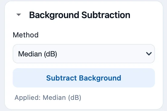
Choose a Method and click Subtract Background. The background is computed for each frequency channel over the whole observation time:
- Mean
-
subtracts the mean of each frequency channel; the result stays in the raw intensity unit (Digits).
- Median
-
subtracts the median of each frequency channel; the result stays in Digits. The median is less affected by bursts and RFI than the mean.
- Median (dB)
-
subtracts the median of each channel and converts the result to decibels above that background, following the CALLISTO Plotutil recipe used by the batch processor. This method is recommended for analysis.
The status line below the button names the method in use, for example Applied: Median (dB). The subtraction is always computed from the raw data, so choosing another method and clicking again replaces the previous result rather than stacking on it. Re-applying the subtraction also clears any RFI cleaning or isolated burst that was derived from the previous result. While a Median (dB) result is shown, the intensity unit is locked to dB because the data are already in decibels. Edit > Reset to Raw removes the subtraction.
Noise Clipping Thresholds
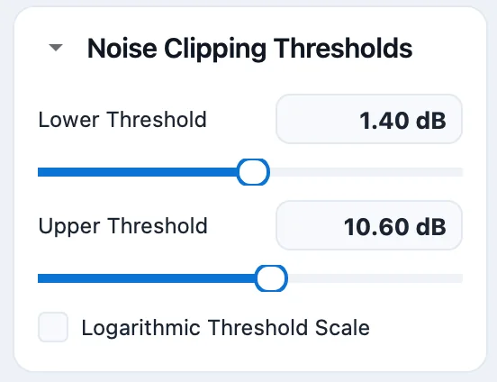
The Noise Clipping Thresholds panel (Figure 6.3) sets the limits of the color scale.
- Lower Threshold / Upper Threshold
-
High-resolution sliders for the lower and upper limits of the color scale (Vmin and Vmax). The display updates live while you drag; no Apply button is needed. The value card beside each label shows the limit. When the intensity is shown in Digits, a second line gives the corresponding dB value.
- Logarithmic Threshold Scale
-
Makes the sliders logarithmic for finer control near zero.
The thresholds change the contrast only; the data are never clipped or modified. With both sliders at zero the color scale spans the whole data range. Limits chosen on the raw data are reset when you subtract the background, because they would saturate the new scale. Processing > Presets > Raw FITS Percentile (5-98%) sets the limits from the distribution of the data on show (Section 7.4).
Units
The Units panel (Figure 6.4) selects the units of the intensity and time axes.
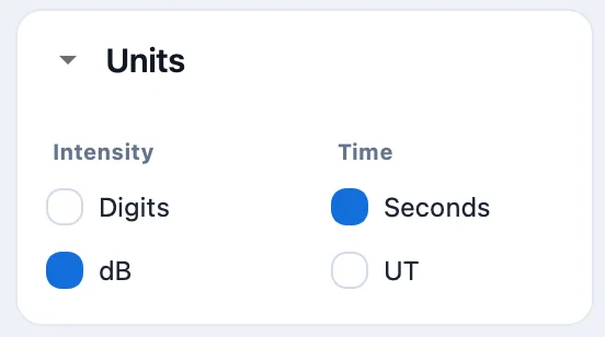
- Intensity: Digits / dB
-
Digits shows raw CALLISTO ADC values as stored in the file. dB converts them with the CALLISTO receiver scale (see the glossary entry Digit).
- Time: Seconds / UT
-
Seconds measures time from the start of the loaded data; UT shows Universal Time. UT requires the observation start time (
TIME-OBS) in the FITS header.
Switching units does not modify or lose data; it only changes the axis labels, the color-bar label and the cursor readout.
Axis
The Axis panel (Figure 6.5) switches the frequency axis between Linear (proportional to MHz) and Log (proportional to MHz).
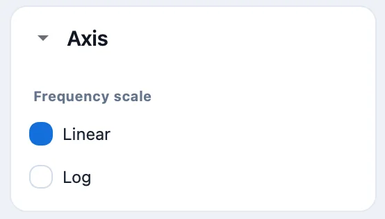
A logarithmic axis spreads out the decametric end of the band, where Type II and Type III bursts spend most of their drift, and places a fundamental–harmonic pair at a constant separation. Ticks are anchored to the decades and labeled in MHz (for example 20, 30, 40, 50, 60, 70, 80 across a 20–80 MHz band), thinning as the span widens. Both renderers support the logarithmic axis, and annotations, the ruler, light-curve picks and drift points behave identically in both scales because their coordinates remain in MHz. The choice is remembered between sessions. The STEREO/SWAVES panel always uses its own logarithmic axis (Section 13.2).
Graph Properties
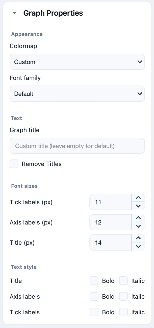
The Graph Properties panel (Figure 6.6) controls the appearance of the plot. It becomes active once a file is loaded. The settings apply to the on-screen plot and to exported figures and reports.
| Group | Control | Function |
|---|---|---|
| Appearance | Colormap | Custom (blue–red–yellow), viridis, plasma, inferno, magma, cividis, turbo, RdYlBu, jet, cubehelix or bone_r. |
| Font family | Typeface of all plot text; Default or any installed font. | |
| Text | Graph title | A custom title; leave empty for the default title. |
| Remove Titles | Hide the plot title. | |
| Font sizes | Tick labels (px) | 6–60 px (default 11). |
| Axis labels (px) | 6–60 px (default 12). | |
| Title (px) | 6–80 px (default 14). | |
| Text style | Title, Axis labels, Tick labels | Bold and Italic for each text element. |
Analysis Summary
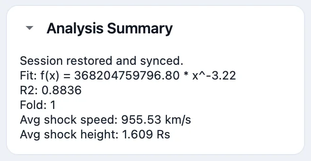
The Analysis Summary panel (Figure 6.7) is a read-only summary of the current analysis session: the fitted equation, , the fold number and the average shock speed and height from the Burst Analyzer (Section 8.7). It also reports when a saved session has been restored. Before any analysis it reads No analysis session loaded.
Ruler Measurement
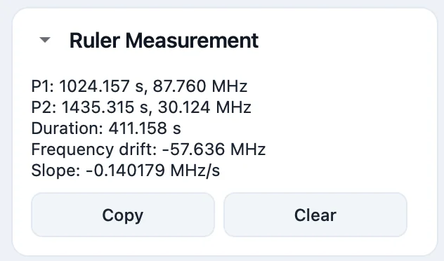
The Ruler Measurement panel (Figure 6.8) shows the result of the ruler tool, started with Analysis > Ruler Measurement (Section 7.8): the two points P1 and P2 (time and frequency), the Duration, the Frequency drift and the Slope in MHz/s. Copy copies the readout to the clipboard and Clear removes the measurement.