Viewing, Processing and Annotation Tools

This chapter describes how to navigate the spectrum, set an exact display range, clean radio-frequency interference, use processing presets, annotate the plot, overlay light curves, and make quick drift-rate and ruler measurements.

Table 7.1 lists the mouse interactions available in the plotting area.

Navigation and picking in the plotting area.
Interaction	How
Zoom	Scroll the mouse wheel over the plot; the zoom is centered on the pointer.
Pan	Hold the left mouse button and drag.
Rectangle zoom	Click Lock zooming and panning on the toolbar, then Rectangular Zooming, and drag a rectangle. Repeat Rectangular Zooming for each further zoom.
Freeze or release the view	Lock zooming and panning disables wheel zoom and panning; Unlock zooming and panning re-enables them.
Cursor readout	Move the pointer over the plot; time, frequency and intensity appear in the status bar.
Estimate drift rate	Click points along the burst; right-click or double-click to finish (Section 7.7).
Isolate burst	Press, drag a loop around the burst and release (Section 8.2).
Ruler	Click two points (Section 7.8).
Light curve by click	With click mode on, click a frequency (Section 7.6).
Annotations	Line: click the start and end. Text: click the position. Polygon: click the vertices and right-click to close (Section 7.5).

Reset Selection clears an isolated-burst selection and drift markers; Reset to Raw discards all processing; Reset All clears the workspace (Table 3.2).

Setting an exact display range

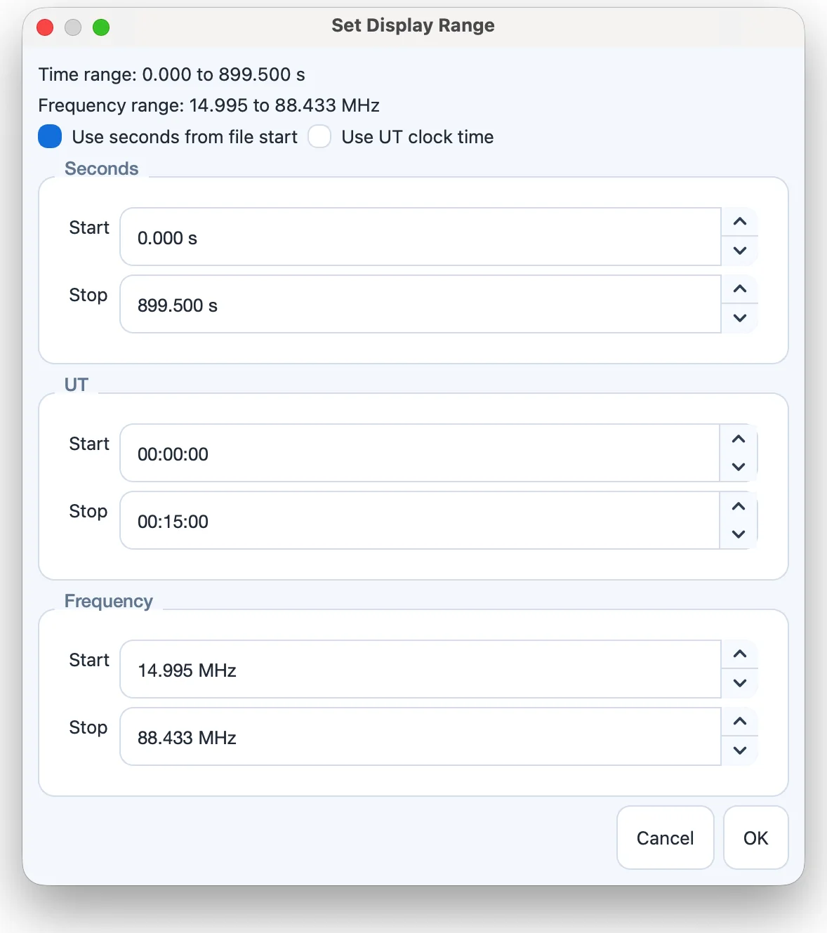
View > Set Display Range... sets the visible window numerically, which is useful for comparing several stations over identical axes (Figure 7.1).

Choose Use seconds from file start or Use UT clock time, then enter the start and stop times in the Seconds or UT group. UT input is unavailable when the file has no TIME-OBS value.
Enter the lower and upper limits in the Frequency group (MHz).
The full time and frequency ranges of the data are shown for reference.

The Set Display Range dialog. — **Figure 7.1.** The **Set Display Range** dialog.

Display-range presets

A display range can be stored under a name with View > Save Display Range Preset..., applied later to another file with Apply Display Range Preset..., and removed with Delete Display Range Preset.... Presets are stored in your preferences and are available in every session.

View configurations

View > Export View Config... saves the display range, units, thresholds, color map and graph styling to a portable .efaview.json file; View > Import View Config... applies such a file. View configurations can be shared with colleagues and are also accepted by the batch processor (Section 10.7) and the Multi-Station Comparison (Chapter 12), so that many spectra can be rendered with identical axes and appearance.

RFI cleaning

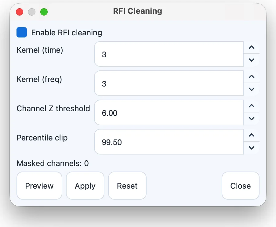
Radio-frequency interference appears as bright horizontal streaks (persistent narrow-band emitters) and short spikes. Processing > RFI Cleaning offers Open RFI Panel, Apply RFI and Reset RFI. The RFI Cleaning panel (Figure 7.2) applies a deterministic pipeline to the dynamic spectrum:

two-dimensional median smoothing with a window of Kernel (freq) $\times$ Kernel (time);
detection of hot channels from a robust $Z$ -score of each channel’s level and variability;
repair of the masked channels from their neighbors;
per-channel clipping of high outliers above an upper percentile (the low side is preserved).

The RFI Cleaning panel. — **Figure 7.2.** The **RFI Cleaning** panel.

RFI cleaning parameters.
Parameter	Range (default)	Effect
Enable RFI cleaning	on/off (on)	Includes RFI cleaning in the processing chain.
Kernel (time)	1–31, odd (3)	Median window along time. Larger values suppress short spikes more strongly but can blur fast burst structure.
Kernel (freq)	1–31, odd (3)	Median window across frequency channels. Larger values reduce narrow-band striping but can widen spectral features.
Channel Z threshold	0.5–20 (6.0)	Cut-off for hot-channel masking. Lower values mask more channels.
Percentile clip	90–99.99 (99.5)	Upper cap applied to each channel. Lower values clip peaks more aggressively.

Preview: shows the result without committing it. The Masked channels line reports the number and indices of the channels flagged as hot.
Apply: commits the cleaning to the processed data.
Reset: restores the default parameters in the panel.
Close: closes the panel.

If channel streaks remain, lower the Channel Z threshold gradually (for example from 6.0 to 5.0 and then 4.0). If burst detail looks over-smoothed, reduce the kernel sizes or raise the threshold. Edit > Reset to Raw reverts all applied processing, including RFI cleaning.

Processing presets

A processing preset stores the display thresholds and their scale, the background subtraction method, the intensity and time units, the color map, the graph styling, the RFI settings and the default annotation style. Presets are managed from Processing > Presets:

Raw FITS Percentile (5-98%): sets the threshold limits to the 5th and 98th percentiles of the data currently shown — a quick starting range for raw files.
Save Current as Preset...: stores the current settings under a name.
Apply Preset...: applies a stored preset to the loaded data.
Set Default Preset...: chooses a preset that is applied automatically to every file loaded afterwards.
Clear Default Preset: stops applying a default preset.
Delete Preset...: removes a stored preset.

Annotations

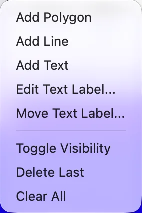
Annotations mark features on the spectrum. They are drawn in both renderers, saved in projects, and included in exported figures and reports. Processing > Annotations (Figure 7.3) contains:

Add Polygon: click the vertices; right-click to close the polygon.
Add Line: click the start point and then the end point.
Add Text: click where the label should go, then enter it in the text dialog.
Edit Text Label...: choose an existing label and change its text and style.
Move Text Label...: choose a label, then click its new position.
Toggle Visibility: show or hide all annotations.
Delete Last: remove the most recent annotation.
Clear All: remove every annotation.

The text dialog sets the Text, Font, Font Size, Font Style (Bold, Italic) and Color of a label.

Light curves

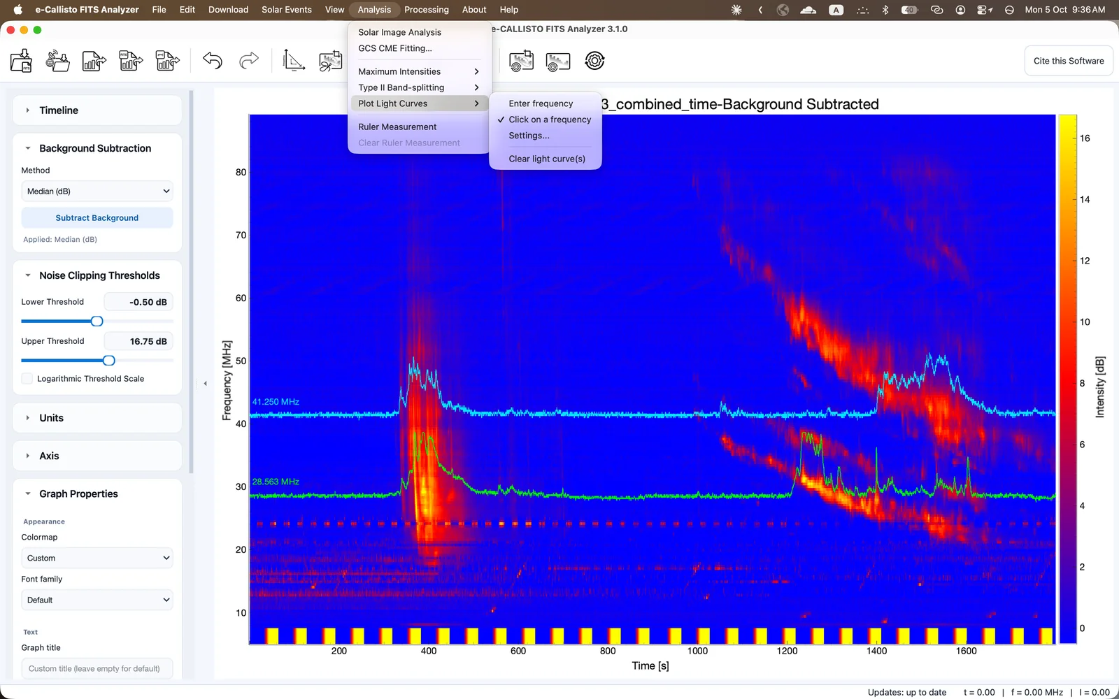
A light curve is the intensity at one frequency as a function of time. Light curves are drawn on top of the spectrum (Figure 7.4) from Analysis > Plot Light Curves:

Enter frequency: opens a dialog for typing a frequency in MHz; the available range of the data is shown.
Click on a frequency: toggles click mode. While it is on, clicking the spectrum plots the light curve at the clicked frequency.
Settings...: opens the Light Curve Settings dialog (Table 7.3).
Clear light curve(s): removes all light curves without affecting the data.

Light curves at two frequencies overlaid on a dynamic spectrum, with the Analysis > Plot Light Curves submenu open. — **Figure 7.4.** Light curves at two frequencies overlaid on a dynamic spectrum, with the **Analysis > Plot Light Curves** submenu open.

Light-curve settings.
Setting	Range	Effect
Mode	Single / Multiple	Single light curve replaces the previous curve; Multiple light curves keeps adding curves.
Color	color picker	Color of the curve.
Thickness	0.5–12	Line width.
Vertical Scale	0.1–5	Height of the curve relative to the plot.
Opacity	0.1–1	Transparency of the curve.
Line Style	solid, dashed, dotted	Line pattern.
Labels	on/off	Show frequency labels next to each curve.

Apply applies the settings, Reset to Defaults restores the defaults and Close closes the dialog. Light curves are saved in projects and can be included in project reports.

Estimating the drift rate

The Estimate Drift Rate toolbar tool gives a quick estimate of a burst’s frequency drift from points that you click.

Click Estimate Drift Rate.
Click two or more points along the burst.
Right-click or double-click to finish.

The points are joined by dashed segments, and the status bar shows the Average Drift Rate in MHz/s (the mean of the segment drift rates), the start and end frequencies, and the duration. Segments of zero duration are ignored. Reset Selection clears the drift markers. For a fitted drift rate and shock parameters, use the Type II analysis tools (Chapter 8).

Ruler measurement

Analysis > Ruler Measurement measures between two points clicked on the spectrum. The readout appears in the sidebar’s Ruler Measurement panel (Section 6.8): the coordinates of both points, the duration, the frequency change and the slope. Analysis > Clear Ruler Measurement or the panel’s Clear button removes it. The ruler is kept when the timeline is extended.

Overlays from other instruments

Two overlays add context directly to the main plot:

the GOES X-ray flux curves, enabled from Solar Events > GOES Overlay (Section 14.3.1); and
the STEREO/SWAVES spectrum below the CALLISTO spectrum (Section 13.2).