Image Display and Processing

This chapter describes the tools of Solar Image Analysis that display, enhance, combine and export image sequences once they are loaded (Chapter 16).

The Analysis card

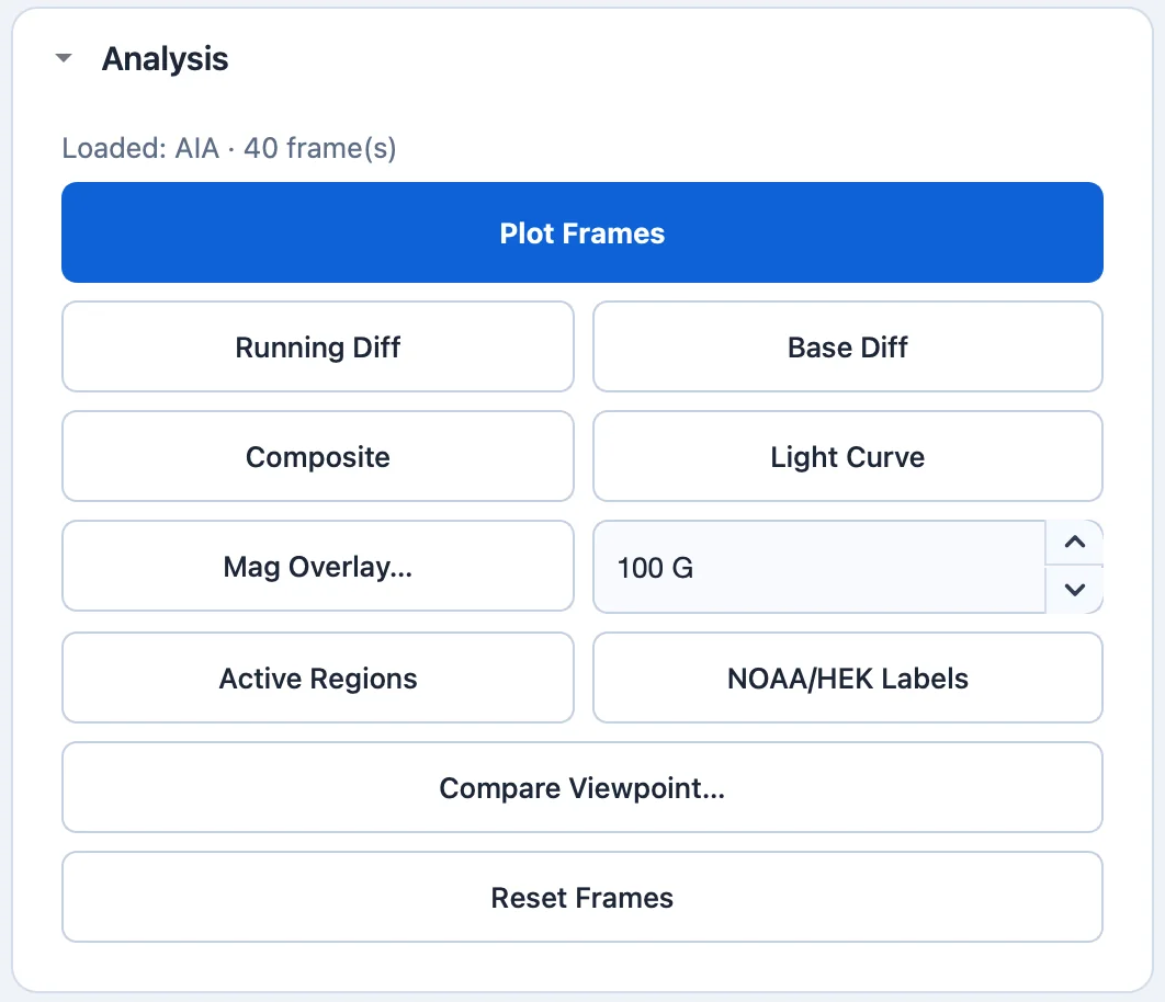
The Analysis card (Figure 17.1a) shows a summary of the loaded data and the main display modes and analysis tools.

(a) Analysis card — **Figure 17.1.** The **Analysis** and **Display & Crop** cards of Solar Image Analysis.

(b) Display & Crop card — **Figure 17.1.** The **Analysis** and **Display & Crop** cards of Solar Image Analysis.

Plot Frames: displays the loaded sequence as plain frames.
Running Diff: displays each frame minus the previous one, which makes moving and changing features stand out.
Base Diff: displays each frame minus the first, showing the total change since the start — useful for eruptions, coronal dimmings and EUV waves.
Composite: builds an RGB tri-color image from the first three AIA frames or, when a magnetogram overlay has been loaded, draws HMI polarity contours on the current AIA frame (red positive, blue negative).
Mag Overlay…: loads an HMI magnetogram FITS file for the composite; the box beside it sets the contour level (10–2000 G; default 100 G).
Light Curve: plots the mean intensity of a region against time (Section 17.4).
Active Regions: , NOAA/HEK Labels detect and label active regions (Section 17.5).
Compare Viewpoint…: compares the frame with a second observer (Section 17.6).
Reset Frames: restores the frames as downloaded, discarding crops, processing levels, derotation, composites and detected regions.

Composite, Mag Overlay…, Active Regions and NOAA/HEK Labels are available only for disk imagers and magnetographs. The difference modes also determine the content of exported movies (Section 17.11).

Display and cropping

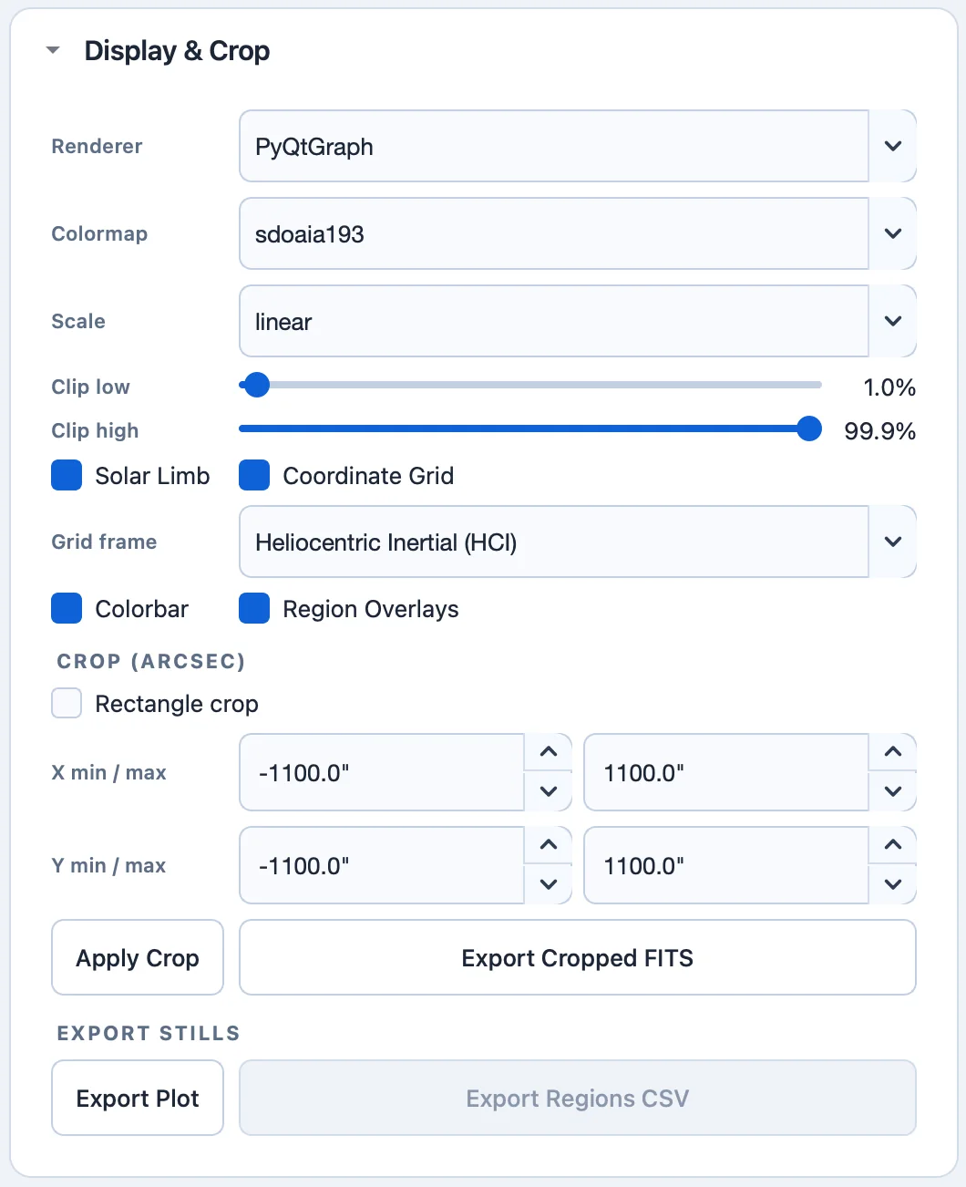
The Display & Crop card (Figure 17.1b) controls the appearance of the image:

Renderer: PyQtGraph (default; fast, and required for clicked PFSS seeds and the interactive crop rectangle) or Matplotlib.
Colormap: instrument color maps (for example sdoaia193, hmimag, soholasco2, stereocor2, euvi195, goes-rsuvi171) and general ones (inferno, magma, plasma, viridis, cividis, gray, RdBu_r, hot). A suitable map is chosen automatically for each observable.
Scale: linear or log.
Clip low, Clip high: the lower and upper percentiles mapped to the ends of the color scale (defaults 1% and 99.9%); dragging gives a live preview.
Solar Limb: draws the photospheric limb.
Coordinate Grid, Grid frame: overlays a graticule of meridians and parallels in the selected frame — Heliocentric Inertial (HCI, the default), Stonyhurst or Carrington. The same frame is used for the heliographic coordinates of the cursor readout.
Colorbar, Region Overlays: show the color bar and the detected active regions.

Cropping

Under Crop (arcsec), enter X min / max and Y min / max in arcseconds from disk center, or tick Rectangle crop to drag a rectangle on the image that fills in the fields. Apply Crop crops all loaded frames to the rectangle. Cropping is done locally after the files are loaded. Export Cropped FITS saves the cropped frames as FITS files with updated coordinate metadata.

The crop rectangle also defines the region used by Region Stats, the light curve, the derotation and the Current crop PFSS seeding.

Solar derotation

Over a sequence of several hours, a fixed rectangle slowly drifts onto neighboring surface because of solar differential rotation. The Solar Derotation card keeps a selected region on the same piece of the Sun:

Derotate selected area: enables derotation of the crop region.
Mode: Track region (no resampling) moves the cut-out window with the rotation and keeps the original pixel values, so it is the mode for photometry and light curves. Reproject to reference time resamples every frame onto the reference time’s grid, which corrects foreshortening and gives all frames one coordinate system, making differencing meaningful, at the cost of interpolating the data.
Reference: First frame, Current frame or Specific frame... (with its number): the frame from which the region is read and to whose time every other frame is rotated.
Padding: the extra margin cut around the region before reprojecting (0–600 arcsec; default 60 arcsec), so that the interpolation has data up to the edge. Reproject mode only.
Apply Derotation, Reset to Full Frames: apply the derotation, or discard the cut-out and restore the full frames at the current processing level.

The status line reports whether derotation is active.

Region light curve

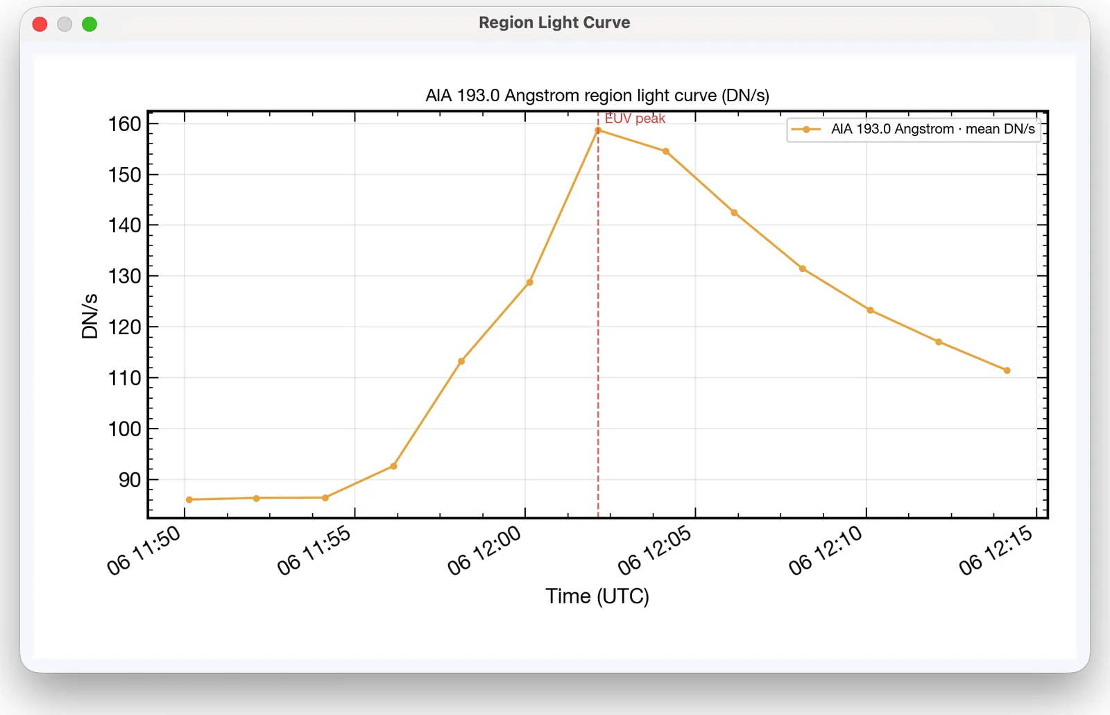
Light Curve plots the mean intensity of the crop region (or of the whole frame if Rectangle crop is off), converted to DN/s using the exposure time, against time (Figure 17.2). The time of peak intensity is marked and, when a spectrum is loaded in the main window, its time window is shaded so that the EUV brightening can be timed against the radio burst. At least two frames are needed.

Active regions

The Active Regions card detects bright regions in the current frame and lists them:

Threshold: the intensity percentile above which pixels count as bright (50–100; default 98).
Min px: the minimum area of a region in pixels (default 12).
Region table: one row per region with ID, Label, NOAA number, Centroid, Area, Peak intensity and Source.

Click Active Regions in the Analysis card to run the detection, and NOAA/HEK Labels to fetch the NOAA active-region numbers from the Heliophysics Event Knowledge base (HEK) and attach them to the detected regions; the status line reports whether metadata are loaded. Detected regions are drawn on the image when Region Overlays is ticked. Export Regions CSV saves the table with centroids, bounding boxes and intensities. Detection works on local files; the labels need network access.

Comparing viewpoints

Compare Viewpoint… opens a window that compares the current frame (viewpoint A) with a second observable (viewpoint B) taken near the same time — for example a STEREO image against the Earth view.

Choose the Second viewpoint observable and the search window (±, 1–720 min; default 30 min).
Click Fetch Viewpoint B. Viewpoint B is downloaded, reprojected onto the coordinate frame of A, and shown beside it.
Tick Blink to alternate between the two images in place.

The Observer separation line gives the angle between the two observers.

Coronagraph tools

For coronagraph data the Coronagraph Tools card offers NRGF radial filter, the normalizing-radial-graded filter (Morgan et al. 2006). It flattens the steep radial fall-off of coronal brightness so that faint CME fronts become visible at all heights. It applies to the plain frame view; difference images already remove the background.

Overlay layers

A CME is never fully visible in one instrument: the eruption starts on the disk (AIA, EIT, EUVI), crosses the low corona (LASCO C2, COR1) and expands into the outer corona (LASCO C3, COR2), and each coronagraph is blind inside its occulter. For coronagraph views the Overlay Layers card blends several instruments into one continuous image from the disk to the outer corona.

Add, Remove: choose an observable and add it to the layer list, or remove the selected layer. Layers are painted widest field of view first. Untick a layer to leave it out without losing its settings.
Per-layer settings: for the selected layer: Colormap, Scale (log or linear), Opacity, Midtones (gamma; 50 suits most solar images), and the Inner and Outer edges of its field of view in $R_\odot$ . Pixels inside the inner edge stay transparent so that the layer below shows through.
Time match: how far from each loaded frame’s time a layer frame may be taken (1–720 min; default 30 min). Widen it for slow cadences or patchy archives.
Build Composite: downloads each layer’s matching frames, reprojects them onto the loaded series and blends them, in the background with a progress bar. The result replaces the view and works with the measurement tools, plot export and movie export.
Clear: drops the composite and restores the originally loaded frames.

Note

Each layer is color-mapped before blending, because EUV disk images and the white-light corona differ by orders of magnitude. Coronagraph layers are reprojected under a spherical-screen assumption, flagged as approximate in the build notes: cross-observer coronagraph overlays are morphological context, not photometry. SOHO/LASCO files carry no observer position, so an Earth-based observer is assumed (accurate to about 1%).

Heliospheric imager J-maps

For STEREO HI1 and HI2 data the Heliospheric Imager (J-map) card builds a time–elongation map (Sheeley et al. 1999):

Background: Median background removes the static F-corona and star field with the per-pixel temporal median; Previous frame uses a running difference.
PA: the position angle of the slit, counter-clockwise from the image $+x$ axis (90° points up; default 90°). Set it along the CME direction.
Build J-map: stacks the slit profiles of all frames into the HI J-map window (elongation in degrees against frame index). An outward-moving CME appears as a slanted bright track.

HMI vector magnetic field

For SDO/HMI data the Magnetic Vector Field (HMI) card overlays the measured photospheric vector field:

Load Vector FITS…: loads the hmi.B_720s field, inclination and azimuth segments of each time step from disk (with the optional disambiguation segment, applied automatically).
Download Vector (JSOC): downloads hmi.B_720s for the query time window through JSOC; this needs the registered JSOC e-mail. Each 720-s time step is four segments of about 50 MB. If no HMI image is loaded, the derived vertical-field ( $B_z$ ) magnetogram is plotted with the vectors.
Show vector field: overlays the field on the HMI frame. The transverse component is drawn as Arrows (length proportional to strength) and/or Streamlines, and |B| layer tints the image by total field strength. Arrows are red where the vertical field points toward the observer ( $+B_z$ ) and blue where it points away.
Spacing, Threshold: the arrow grid spacing (16–512 detector pixels; default 64) and the minimum transverse field drawn (50–2000 G; default 200 G). The transverse noise floor of hmi.B_720s is about 100 G.

Movies and still images

Movie Export card: choose the Content (Frames, Running Difference or Base Difference) and the Format (MP4 or GIF), and click Build Movie…. Movies use the playback speed set under the viewer and the current color map, scale, clipping and crop.
Export MP4: in the header bar makes a one-click MP4 of the loaded sequence with the current display settings.
Export Plot: saves the current frame, with its overlays, as an image.
Export Cropped FITS: saves the cropped frames as FITS files.
Export Regions CSV: saves the active-region table.

The same exports are available from the Export and Movie menus.