Fitting the Flux Rope and the Shock

This chapter describes the models of the GCS CME Fitting window, how they are aligned and refined against the observed fronts, how fits are recorded over time to build kinematics, and how results are exported.

The Model card

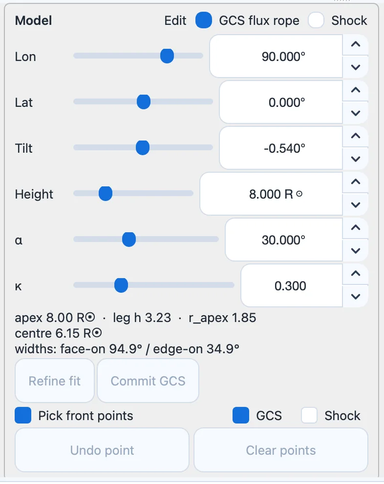
The Model card (Figure 21.1) shows the parameters of one model at a time. Choose the model with Edit on the card’s title row:

GCS flux rope: the Graduated Cylindrical Shell, fitted to the CME ejecta.
Shock: a spheroid or ellipsoid, fitted to the shock the CME drives — its faint outer envelope (Section 21.7).

Both models are drawn in every panel (the shell in orange and the shock in sky blue by default); the edited model is the one that the handles, clicks, Refine fit, Commit and the Kinematics card act on.

GCS parameters

Six sliders, each with a numeric entry, control the shell (Table 21.1).

Parameters of the GCS flux-rope model.
Slider	Range	Meaning
Lon	$-180^\circ$ to $180^\circ$	Stonyhurst longitude of the direction of propagation.
Lat	$-89^\circ$ to $89^\circ$	Stonyhurst latitude of the direction of propagation.
Tilt	$-90^\circ$ to $90^\circ$	Rotation of the shell about the propagation direction.
Height	1.05–30 $R_\odot$	Distance of the leading edge (apex) from Sun center — not the altitude above the surface.
$\alpha$	$1^\circ$ – $80^\circ$	Half-angle between the legs of the shell.
$\kappa$	0.05–0.95	Aspect ratio, controlling the thickness of the shell.

Set the direction, tilt, $\alpha$ and $\kappa$ before fine-tuning the height. The apex can also be dragged in any panel: moving it around the Sun turns the direction, and moving it outwards or inwards changes the height. The readout below the sliders gives the derived leg height, apex cross-section radius, center distance, and the intrinsic face-on and edge-on widths.

Background: GCS geometry

The GCS is a hollow croissant: two conical legs joined by a curved front with a circular cross-section that grows with distance from the Sun (Thernisien et al. 2006; Thernisien 2011). The face-on width is $2[\alpha + \arcsin\kappa]$ and the edge-on width $2\arcsin\kappa$ ; both include the shell thickness and differ from the apparent width in a coronagraph image. Because the height is the leading edge, it feeds the height–time fit directly. GCS is a flux-rope model, not a shock model.

Clicking the front

With Pick front points ticked, left-click points along the same front in two or more views. Points are drawn in each panel and are used by Refine fit:

a right-click removes that panel’s last point;
Undo point (Ctrl+Z) removes the point clicked last in any panel;
Clear points removes all of the edited model’s points on the displayed images;
untick Pick front points to navigate without adding points.

The GCS wireframe and Shock wireframe options hide a model temporarily so that the observed front can be inspected. Each model keeps its own front points.

Refining the fit

Refine fit (Ctrl+R) makes a local least-squares adjustment of the edited model through the clicked points. It refines a fit; it cannot find one from scratch, because longitude, $\alpha$ and $\kappa$ are poorly conditioned in GCS, so first align the shell roughly with the CME by eye. The refinement fits as many parameters as the points support (Table 21.2); the status bar names the parameters fitted and how many more points would free the next one.

Staged refinement of the GCS model.
Front points	Parameters fitted
2	Height
4, in two separated views	Height, longitude, latitude
5	…and tilt
6	…and $\alpha$
7	All six parameters (adding $\kappa$ )

The status bar also reports the views taking part, their angular separations and the number of points. Only images within the Max time offset of the shared time take part. With a single view, or with no pair of views between 20° and 160° apart, the direction cannot be constrained and is held fixed; empty, nearly coincident and nearly opposite viewpoints do not constrain the direction independently. Formal errors are shown when the local solution is reliable, are withheld otherwise, and become invalid when the model or the observations change.

Recording fits

Commit GCS (Ctrl+Return) records the current fit at the shared time, together with the images it was made from and their observation details. Step to later times and repeat to build a height–time series. One combination of images cannot be recorded at two different times, so repeated images never count as independent height measurements.

When stepping, dragging the time slider or playing, the recorded shells are drawn: each fit on its own images, interpolated between recorded times (a display, not a fit) and held before the first and after the last record. A model with nothing recorded keeps its slider values, so commit before stepping away. Fit > Restore recorded model at current time and Delete recorded fit at current time revisit or remove a record; Fit > Reset model parameters resets the edited model.

Moving the event range to a different event sets the recorded fits aside. They return when you come back to that event, and the JSON export includes them.

Kinematics

The Kinematics card (Figure 21.2) lists the recorded fits of the edited model beside a height–time graph. For the GCS model the table shows Time (UT), t (s), Apex (R☉), Lon (°), Lat (°) and α (°); for the shock, $\kappa$ replaces $\alpha$ .

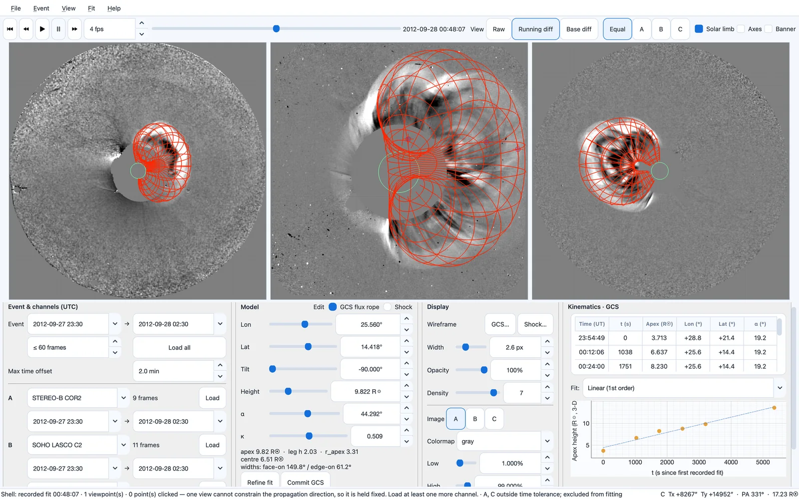
Double-click a row to go back to its time and restore its model.
Choose a Linear, Quadratic or Cubic fit and click Fit height–time. A fit of degree $n$ needs $n+1$ recorded times, and $n+2$ before errors can be estimated (Section 18.4).
Clear fits removes the recorded fits of the edited model.
Export saves the table as CSV or the graph as a figure.

The heights are de-projected under the model assumptions, so the speeds are model-dependent radial speeds rather than plane-of-sky speeds.

Fitting the shock

Choose Edit: Shock to fit the shock with a Spheroid or an Ellipsoid (Figure 21.3). The parameters follow PyThea’s conventions exactly (Table 21.3).

Parameters of the shock model.
Slider	Range	Meaning
Lon, Lat	as for GCS	Stonyhurst direction of the shock center and apex.
Height	1.05–30 $R_\odot$	Heliocentric distance of the apex (center distance plus the radial semi-axis $a$ ).
$\kappa$	0.05–2.0	Self-similar constant $\kappa = b/(h - 1\,R_\odot)$ : the lateral size for a given apex height.
$\varepsilon$	$-0.99$ to $0.99$	Signed eccentricity: positive stretches the shock radially ( $a > b$ ), negative flattens it ( $a < b$ ).
Tilt	$-90^\circ$ to $90^\circ$	Ellipsoid only: rotation about the radial axis; at 0 the $b$ axis is parallel to the solar equator.
$\alpha$ (b/c)	0.5–1.5	Ellipsoid only: ratio of the two lateral semi-axes.

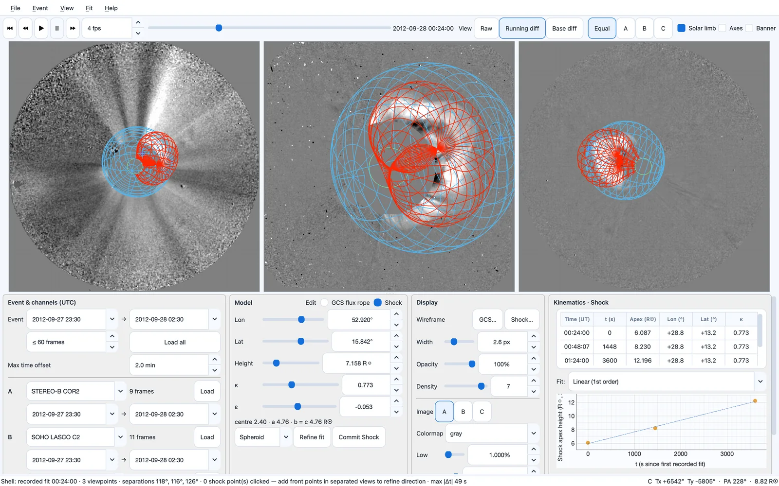
**Figure 21.3.** Shock and flux-rope models in three viewpoints.

The derived readout gives the center distance and the semi-axes, under PyThea’s names. Click the shock front and use Refine fit: the model’s exactly computed projected outline is pulled through the points in every view, with its own sequence of height, direction and shape parameters. Record shock fits with Commit Shock. The shock keeps its own front points, recorded fits, kinematics and CSV file. With fewer than three views, $\varepsilon$ and the tilt are weakly constrained and an ellipsoid’s shape parameters trade off against each other, so prefer a spheroid.

Exporting results

Images and graphs are drawn again from the data rather than copied from the screen, always on a white page whatever the application theme; graphs follow the OriginPro style. Figures can be saved as PNG, PDF, EPS, SVG, TIFF or JPG.

Export analysis JSON…: (Ctrl+Shift+S) the current, recorded and set-aside parameters of both models, with the clicked points, image times, offsets and observer geometry. The file (schema version 2) has a shock section beside the GCS keys. It is an analysis export, not a PyThea session file.
Export recorded fits CSV…: the recorded series of the edited model (cme_gcs_fit.csv or cme_shock_fit.csv).
Export height–time graph…: the recorded apex heights with error bars and the chosen fit, titled with the model and fit, with the speed and acceleration in the legend.
Save viewpoint snapshot…: the three views as shown, with arcsecond axes, the wireframes, the solar limb, the front points and a note of where each drawn shell comes from. With the banners hidden, only each panel’s name is printed above it.
Export movie (GIF/MP4)…: every time step as playback shows it, recorded shells included, at the playback speed. MP4 needs the bundled FFmpeg; a GIF is offered when it is unavailable.
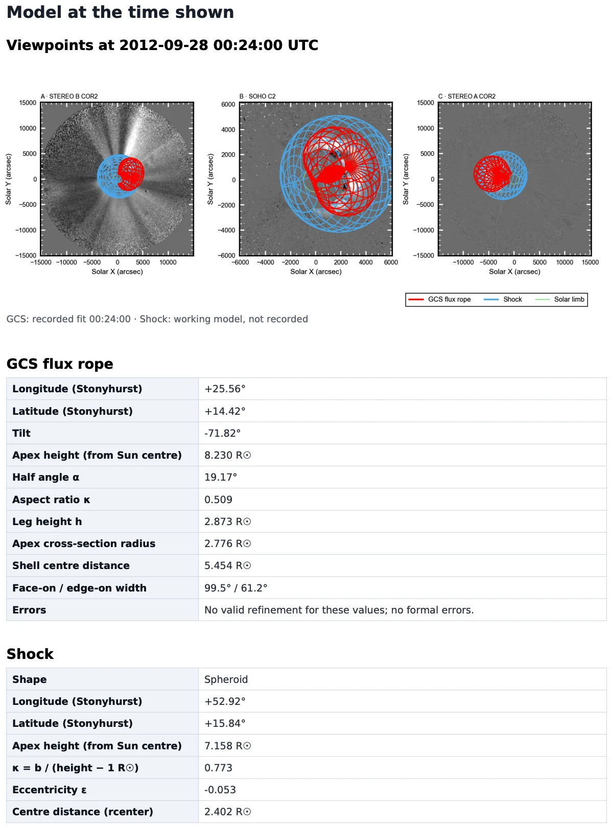
Export fitting report (PDF)…: the viewpoints and their separations, the model at the current time, every recorded fit drawn on the images it was made from with its parameters and observation details, each model’s linear, quadratic and cubic height–time fits (each with a titled graph and all its parameters, then compared), and the method, its limits and references (Figure 21.4).

Stepping through time for a movie or a report leaves the window as it was: the time shown, the working models, their formal errors and the front points are restored afterwards.

**Figure 21.4.** A page of the GCS fitting report.

Scientific limits

GCS models the flux rope, not the shock. Formal fit errors leave out the uncertainty from identifying the front, non-simultaneous images, image preparation and the assumed geometry, and a small residual does not make a fit unique or accurate (Verbeke et al. 2023). Helioviewer JPEG2000 images are display products: suitable for fitting shapes, not for calibrated intensity measurements. Help > Fitting workflow and scientific limits… (F1) summarizes the procedure and these limits.