Type II Band-Splitting Analysis

The emission lanes of many Type II bursts are split into two parallel bands, interpreted as emission from the plasma ahead of (upper band) and behind (lower band) the shock front. The frequency ratio of the two bands gives the shock’s density compression ratio, from which the Alfvén Mach number, the Alfvén speed and the coronal magnetic field can be estimated (Vršnak et al. 2002). The Type II Band-splitting window performs this analysis directly on the current noise-reduced dynamic spectrum.

Opening the window

Open the window with Analysis > Type II Band-splitting > Open Type II Band-splitting. The calculation needs the shock speed and the starting frequency from the Burst Analyzer, so run the Analyzer (Section 8.7) first. The Analyzer Reference panel reports Analyzer reference data loaded. when these values are available, and Analyzer input missing. otherwise.

Window layout

The tools and panels of the window are numbered in Figure 9.1 and described in Table 9.1.

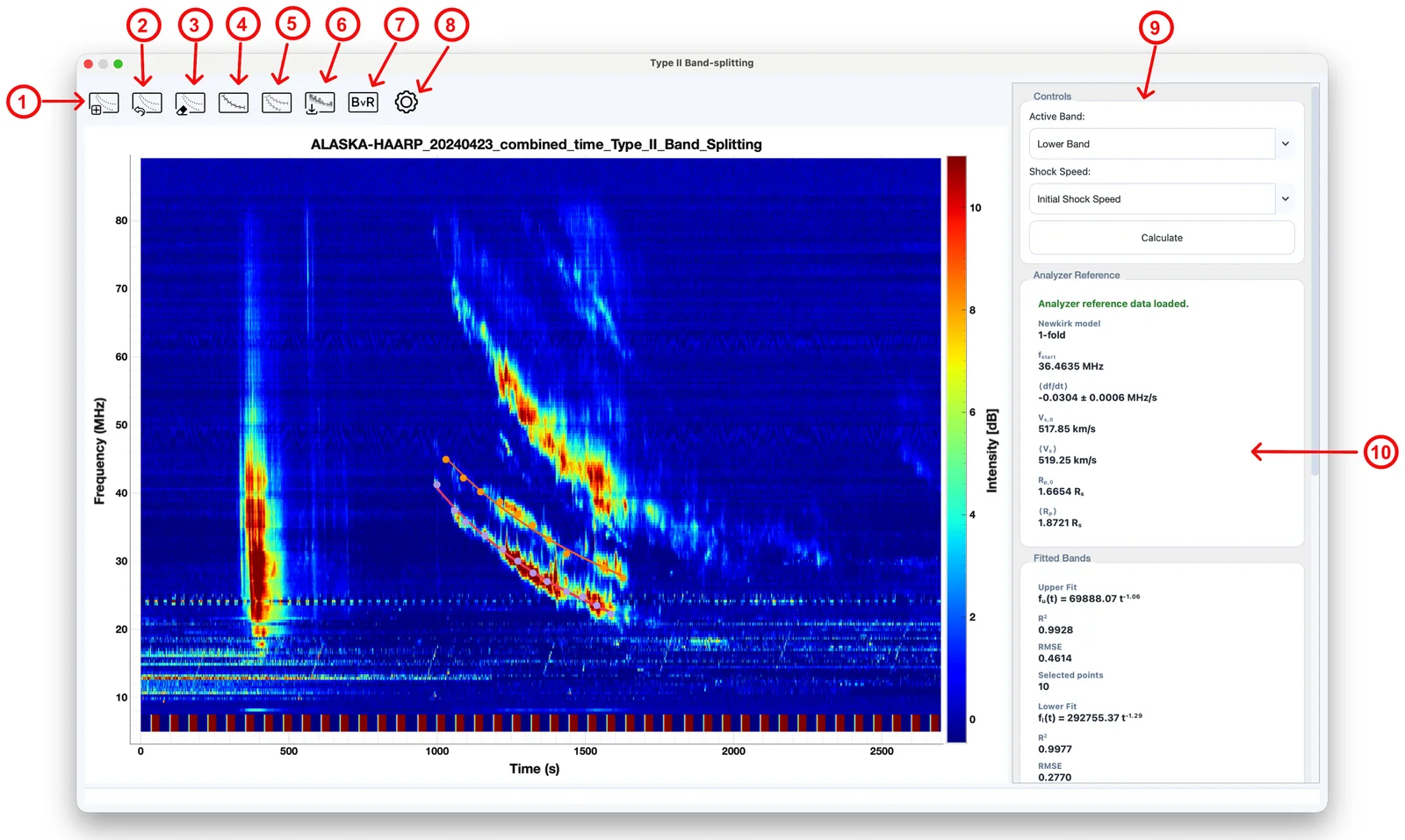
**Figure 9.1.** The Type II Band-splitting window with its tools and panels numbered.

Tools and panels of the Type II Band-splitting window.
No.	Tool or panel	Function
1	Add Points	Toggle point picking; click along the active band on the spectrum to add points.
2	Undo Last Point	Remove the last point added to the active band.
3	Clear Active Band	Remove all points of the active band.
4	Fit Active Band	Fit the points of the active band with a power law.
5	Fit Both Bands	Fit the upper and the lower band.
6	Save Plot	Save the fitted lanes over the spectrum, or the magnetic field versus height plot, as a figure.
7	BvR	Toggle the plot of magnetic field versus shock height (Section 9.5).
8	Settings	Graph settings: fonts, lane colors, line widths and marker sizes (Section 9.6).
9	Controls panel	Active Band (Upper Band or Lower Band), Shock Speed (Initial Shock Speed or Average Shock Speed) and Calculate.
10	Results panels	Analyzer Reference, Fitted Bands and Averaged Band-Splitting Quantities (Section 9.4).

Picking and fitting the bands

Select the Active Band in the Controls panel 9.
Switch on Add Points 1 and click points along that band on the spectrum. Points of the upper and lower bands are drawn in different colors.
Select the other band and add its points.
Fit each band with Fit Active Band 4, or both at once with Fit Both Bands 5.

Each band is fitted with a power law $f(t) = a\,t^{-b}$ , where $t$ is measured from the start of the file. At least two points with positive time and frequency are needed per band. The Fitted Bands panel shows each fitted equation, $R^2$ , RMSE and the number of selected points.

Calculation and results

Choose whether the Initial Shock Speed or the Average Shock Speed from the Analyzer is used, and click Calculate. The results panels contain:

Analyzer Reference: the reference values imported from the Burst Analyzer: the fold number, the starting frequency $f_\mathrm{start}$ , the average drift rate $\langle\mathrm{d}f/\mathrm{d}t\rangle$ , the initial and average shock speeds $V_{s,0}$ and $\langle V_s\rangle$ , and the initial and average shock heights $R_{p,0}$ and $\langle R_p\rangle$ .
Fitted Bands: the fitted equation, $R^2$ , RMSE and number of points of each band.
Averaged Band-Splitting Quantities: the averaging interval, the start time $t_\mathrm{start}$ and band frequencies, the mean upper and lower frequencies, the bandwidth $\langle\Delta f\rangle = \langle f_u - f_l\rangle$ , the mean upper-band drift $\langle\mathrm{d}f_u/\mathrm{d}t\rangle$ , the compression ratio $X = (\langle f_u\rangle/\langle f_l\rangle)^2$ , the Alfvén Mach number $M_A$ , the Alfvén speed $V_A$ and the magnetic field $B$ .

The averaging interval is the time span of the upper-band points; the two fitted curves are sampled over it. If the lower-band fit has to be extrapolated over part of the interval, a warning is shown. The calculation is refused if the compression ratio does not stay between 0 and 4 over the interval.

Background: band-splitting relations

For a perpendicular shock in a low- $\beta$ plasma the compression ratio $X$ and the Alfvén Mach number are related by (Vršnak et al. 2002) $\begin{equation*} X = \left(\frac{f_u}{f_l}\right)^2, \qquad M_A = \sqrt{\frac{X\,(X+5)}{2\,(4-X)}}. \end{equation*}$ The Alfvén speed follows from the shock speed $V_s$ taken from the Analyzer, $V_A = V_s/M_A$ , and the magnetic field from $B = V_A\sqrt{\mu_0\,m_p\,n_e}$ , with the electron density obtained from the plasma frequency, $n_e = (f/8.98\times10^{-3}\,\mathrm{MHz})^2$ cm $^{-3}$ . In the averaged result the density is taken at the Analyzer’s starting frequency.

Magnetic field versus height

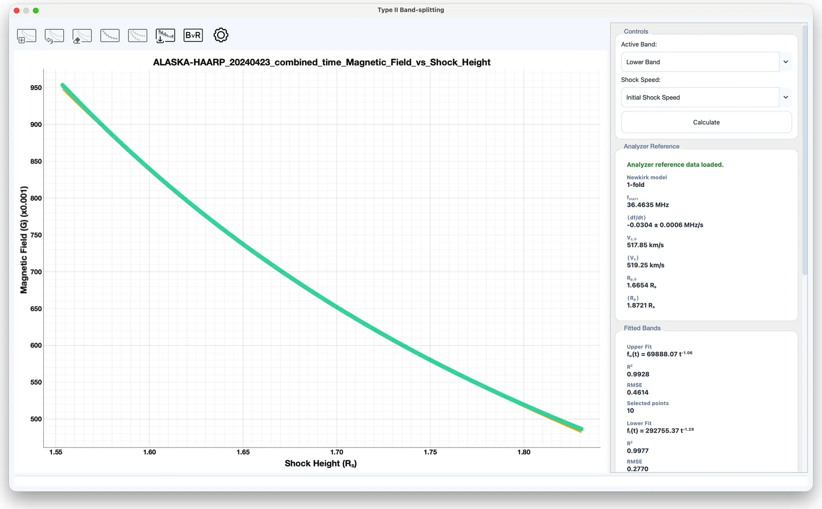
After a successful calculation, the BvR tool 7 plots the magnetic field against shock height (Figure 9.2). Along the averaging interval the field is computed at each sample time from the local compression ratio, with the density taken from the upper-band frequency. The heights are calculated with the Newkirk model and the Analyzer’s fold number, and the profile is fitted with a power law $B = a\,R^{-b}$ . Click BvR again to return to the spectrum.

**Figure 9.2.** Magnetic field versus shock height in the band-splitting window.

Note

The shock speed is taken from the Burst Analyzer and therefore follows the density model selected there (Section 8.7.3). The heights of the magnetic field versus height profile always use the Newkirk model, with the fold number set in the Analyzer.

Graph settings

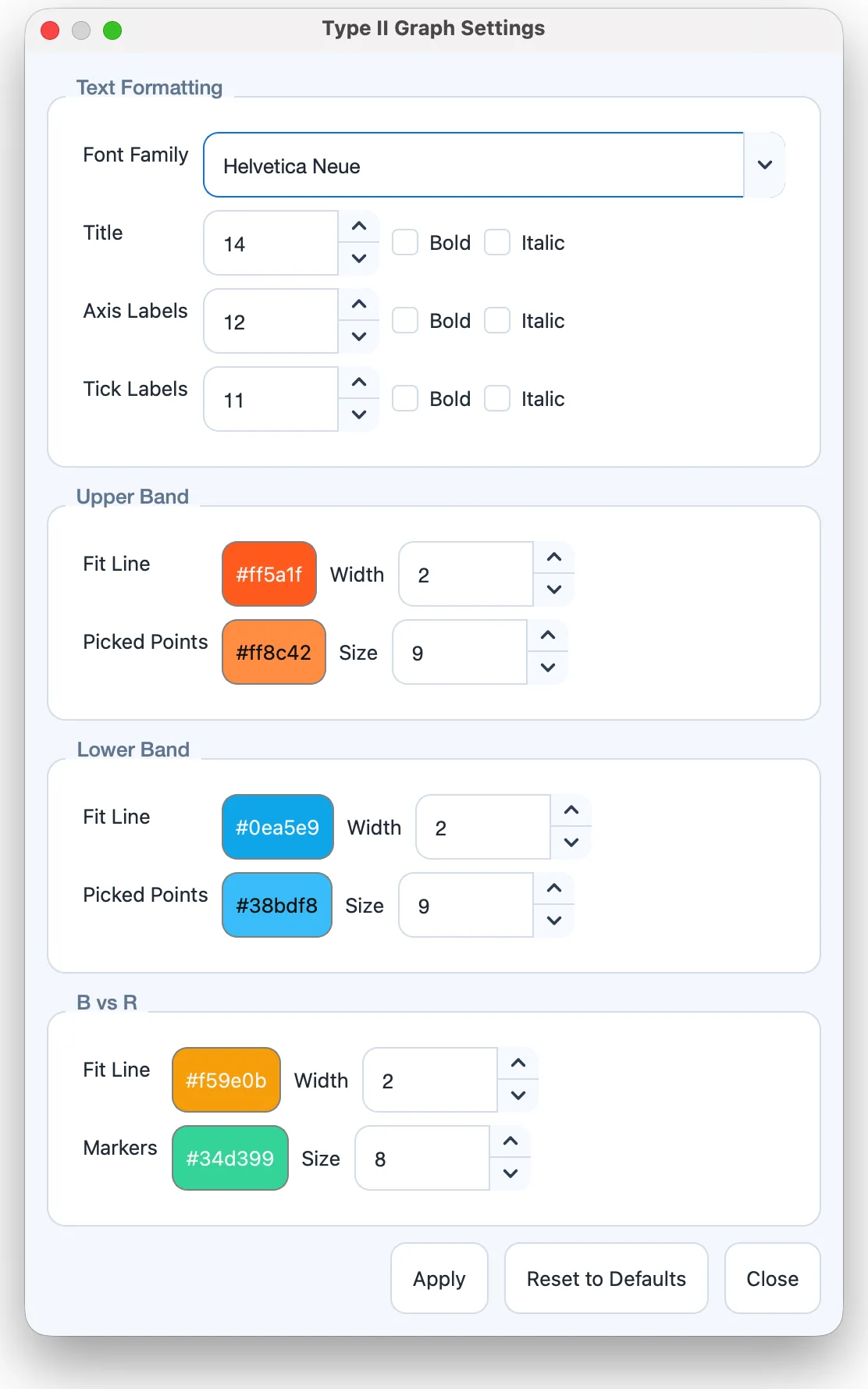
The Settings tool 8 opens the Type II Graph Settings dialog (Figure 9.3):

Text Formatting: font family, and size, bold and italic for the title, the axis labels and the tick labels.
Upper Band, Lower Band: color and width of the fit line, and color and size of the picked points.
B vs R: color and width of the fit line, and color and size of the markers.

Apply applies the settings, Reset to Defaults restores the defaults and Close closes the dialog.

The Type II Graph Settings dialog. — **Figure 9.3.** The **Type II Graph Settings** dialog.

Saving plots

Save Plot 6 exports either the fitted lanes over the dynamic spectrum or the magnetic field versus height fit, whichever is on show, as an OriginPro-style graph in PNG, PDF, EPS, SVG, TIFF or JPG format. The lane colors and fonts from the graph settings are kept.

Caution

Derived magnetic-field values may not be accurate for all events or under all assumptions. They depend on the shock geometry, the density model and the interpretation of the split bands. Confirm results against known or independently validated events before using them for scientific conclusions.