The Main Window

The main window is where dynamic spectra are displayed, processed and measured, and from where every other tool is opened. This chapter describes its layout, toolbar, menus and status bar. The sidebar panels are described in Chapter 6.

Layout

The main window (Figure 3.1) consists of the regions listed in Table 3.1.

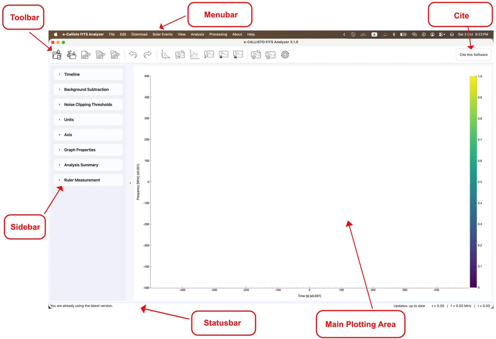
**Figure 3.1.** Main window of the e-CALLISTO FITS Analyzer before a file is loaded.

Regions of the main window.
Region	Description
Menu bar	Access to every function, including those not on the toolbar (Section 3.4). On macOS the menu bar is at the top of the screen.
Toolbar	Icon buttons for the most frequent actions (Section 3.2).
Cite this Software	Opens the citation dialog (Section 4.2).
Sidebar	Collapsible panels for the timeline, background subtraction, display thresholds, units, axis scale, graph properties, the analysis summary and the ruler readout (Chapter 6).
Main plotting area	The dynamic spectrum with its color bar. Interactive tools act here.
Status bar	Messages on the left; the update status and the live cursor readout on the right (Section 3.5).

A narrow arrow handle on the left edge of the plotting area hides or shows the sidebar to give the plot more room. The divider between the sidebar and the plot can also be dragged.

The toolbar (Figure 3.2) contains 16 tools, described in Table 3.2. Hovering over a tool shows its name. Tools that need loaded or processed data remain disabled until they can be used.

Toolbar tools.
No.	Tool	Function	Shortcut
1	Open / Load	Load one or more CALLISTO FITS files from disk (Section 5.2).	`Ctrl+O`
2	Download	Open the e-CALLISTO FITS Downloader (Chapter 11).
3	Export	Export the displayed spectrum as a figure (Section 10.3).	`Ctrl+E`
4	Export as FITS	Export the processed spectrum as a FITS file (Section 10.4).	`Ctrl+F`
5	Save Project	Save the complete workspace as an `.efaproj` project (Section 10.1).	`Ctrl+S`
6	Undo	Undo the last processing change.	`Ctrl+Z`
7	Redo	Redo the last undone change.	`Ctrl+Shift+Z`
8	Estimate Drift Rate	Estimate the drift rate from points clicked along a burst (Section 7.7).
9	Isolate Burst	Draw a freehand mask around a burst (Section 8.2).
10	Plot Maximum Intensities	Open the Maximum Intensities window (Section 8.3).
11	Rectangular Zooming	Drag one rectangle to zoom into the plot. Available while navigation is locked (Section 7.1).
12	Lock zooming and panning	Disable scroll-wheel zooming and panning, freezing the view and enabling rectangle zoom.
13	Unlock zooming and panning	Re-enable scroll-wheel zooming and panning.
14	Reset Selection	Clear the isolated-burst selection and drift markers.
15	Reset to Raw	Discard all processing and show the raw spectrum.
16	Reset All	Clear the workspace: data, processing, selections and analysis overlays.

Caution

Reset All clears the whole workspace. Save a project first if you want to keep the current state.

Plotting area and renderers

The plotting area shows the dynamic spectrum with frequency on the vertical axis, time on the horizontal axis and intensity as color. The plot title shows the source file name and the processing state, for example -Background Subtracted or -Isolated Burst.

Two renderers are available and are selected with View > Mode:

Modern: uses a hardware-accelerated canvas (PyQtGraph) for fast zooming and panning of large or combined spectra. This is the default.
Classic: uses Matplotlib.

Processing > Hardware Acceleration > Enable switches the accelerated live canvas on or off. Both renderers support the same tools, annotations and overlays, and exported figures look the same whichever renderer is in use (Section 10.3).

Menu bar

Table 3.3 summarizes the menus of the main window. The tables that follow list every command, with its shortcut and the section where it is described.

Menus of the main window.
Menu	Main functions
File	Open and combine FITS files; recent files and projects; open, save and recover projects; project reports; figure, FITS, provenance and analysis-log export.
Edit	Undo and redo; extend the timeline with adjacent observations; reset to raw data; reset the workspace.
Download	Launch the e-CALLISTO FITS Downloader.
Solar Events	CME catalog, GOES X-ray and proton flux, geomagnetic indices, SunPy Explorer, radio-burst downloaders, time-window synchronization, GOES overlay and the SWAVES panel.
View	FITS header, display range and its presets, view configurations, Multi-Station Comparison, theme and rendering mode.
Analysis	Solar Image Analysis, GCS CME Fitting, maximum intensities, Type II band-splitting, light curves and the ruler.
Processing	Hardware acceleration, RFI cleaning, annotations, presets, automatic outlier cleaning, restored analysis sessions and batch processing.
About	Update check, bug report and version information.
Help	The built-in user guide.

File menu.
Command	Function	Shortcut, see
Open	Load one file, or combine a compatible multi-file selection.	`Ctrl+O`, §5.2
Recent Files	Reopen one of the last ten FITS selections.	§5.2.1
Combine FITS Files...	Validate, preview and import time, frequency or time $\times$ frequency combinations.	§5.4
Open Project...	Open a saved `.efaproj` project.	`Ctrl+Shift+O`, §10.1
Recent Projects	Reopen one of the last ten projects.	§10.1
Save Project	Save the workspace to the current project file.	`Ctrl+S`
Save Project As...	Save the workspace to a new project file.	`Ctrl+Shift+S`
Recover Last Session...	Restore the most recent autosave snapshot.	§10.2
Generate Project Report...	Create a PDF summary of the dataset and analysis.	§10.6
Export As > Export Figure	Save the plot as an image or vector figure.	`Ctrl+E`, §10.3
Export As > Export to FIT	Save the processed spectrum as a FITS file.	`Ctrl+F`, §10.4
Export As > Export Provenance Report...	Write Markdown and JSON provenance summaries.	§10.5
Export As > Export Analysis Log...	Write CSV and text summaries of the fit and shock results.	§10.5

Note

The disabled File > Save As entry in the main window is reserved; projects are saved with Save Project and Save Project As....

Edit menu.
Command	Function	Shortcut, see
Undo	Undo the last processing or timeline change.	`Ctrl+Z`
Redo	Redo the last undone change.	`Ctrl+Shift+Z`
Add Previous Observation	Prepend the preceding 15-minute observation.	`Ctrl+Shift+Left`, §6.1
Add Next Observation	Append the following observation.	`Ctrl+Shift+Right`, §6.1
Prefetch Adjacent Observations	When ticked (default), download neighboring observations in the background so the next timeline step is instant.	§6.1
Reset to Raw	Remove all processing and return to the loaded data.
Reset All	Clear processing, selections, analysis overlays and the loaded data.

Download and Solar Events menus.
Command	Function	See
Download > Launch FITS Downloader	Open the e-CALLISTO FITS Downloader.	Ch. 11
Solar Events > CMEs > SOHO/LASCO CME Catalog	Daily CME lists, parameters and movies.	§14.7
Solar Events > Flares > GOES X-Ray Flux	GOES XRS viewer and flare parameters.	§14.3
Solar Events > Energetic Particles > GOES SEP Proton Flux	GOES SGPS proton flux viewer.	§14.4
Solar Events > Geomagnetic > Kyoto Dst Index	Dst index viewer.	§14.5
Solar Events > Geomagnetic > GFZ Kp Index	Kp index viewer.	§14.6
Solar Events > Archives > SunPy Multi-Mission Explorer	Multi-mission archive search and plotting.	Ch. 15
Solar Events > Radio Bursts > e-CALLISTO	The e-CALLISTO FITS Downloader.	Ch. 11
Solar Events > Radio Bursts > Learmonth	Learmonth spectrograph browser.	§13.1
Solar Events > Radio Bursts > SWAVES	STEREO/SWAVES loader.	§13.2
Solar Events > Sync Current Time Window	Send the time range of the loaded spectrum to open context windows.	§14.2
Solar Events > GOES Overlay > Short(XRS-A), Long(XRS-B)	Draw GOES X-ray curves on the spectrum.	§14.3.1
Solar Events > SWAVES Panel	Show or hide the loaded SWAVES panel.	§13.2

View menu.
Command	Function	See
View FITS Header	Show the primary header of the loaded file.	§5.5
Set Display Range...	Enter exact time and frequency limits.	§7.2
Save / Apply / Delete Display Range Preset...	Store and reuse named display ranges.	§7.2
Export View Config..., Import View Config...	Share display settings as `.efaview.json`.	§7.2.2
Multi-Station Comparison...	Open the comparison workspace.	Ch. 12
Theme > System / Light / Dark	Choose the color theme.	§3.6
Mode > Classic / Modern	Choose the Matplotlib or hardware-accelerated renderer.	§3.3

Analysis menu.
Command	Function	See
Solar Image Analysis	Open the multi-mission imaging workspace.	Ch. 16
GCS CME Fitting…	Open the GCS window for the visible time range.	Ch. 20
Maximum Intensities > Open Maximum Intensities	Extract the peak frequency of each time channel.	§8.3
Type II Band-splitting > Open Type II Band-splitting	Open the band-splitting analyzer.	Ch. 9
Plot Light Curves > Enter frequency	Plot a light curve at a typed frequency.	§7.6
Plot Light Curves > Click on a frequency	Toggle click mode for light curves.	§7.6
Plot Light Curves > Settings...	Light-curve appearance.	§7.6
Plot Light Curves > Clear light curve(s)	Remove all light curves.	§7.6
Ruler Measurement	Measure duration, frequency change and slope between two points.	§7.8
Clear Ruler Measurement	Remove the ruler.	§7.8

Processing, About and Help menus.
Command	Function	Shortcut, see
Processing > Hardware Acceleration > Enable	Toggle the accelerated live canvas.	§3.3
Processing > RFI Cleaning > Open RFI Panel / Apply RFI / Reset RFI	RFI cleaning pipeline.	§7.3
Processing > Annotations > …	Polygon, line and text annotations.	§7.5
Processing > Presets > …	Processing presets and the default preset.	§7.4
Processing > Maximum Intensity > Auto-Clean Isolated Burst Outliers	Remove outliers automatically when maxima are taken from an isolated burst.	§8.5
Processing > Analysis Session > Open Restored Analysis	Reopen the analysis windows of a restored session.	§10.1.1
Processing > Batch Processing > Open Batch Processor	Export many files with consistent settings.	§10.7
About > Check for Updates...	Look for a newer release.	§4.3
About > Report a Bug...	Prepare a bug report with diagnostics.	§4.4
About > About	Version and author information.	§4.5
Help > User Guide	Open the built-in user guide.	`F1`, §4.1

Status bar

The left part of the status bar shows messages from the current operation, for example the result of a drift-rate estimate or a reminder of how to finish a tool. The right part shows:

the update status, for example Updates: up to date; and
the live cursor readout t = … | f = … MHz | I = …, giving the time, frequency and intensity (in the selected units) under the mouse pointer.

The readout allows quick quantitative inspection of the spectrum without clicking.

Themes

View > Theme selects System (follow the operating system), Light or Dark. The theme applies to all windows of the application and to on-screen plots. Exported figures and PDF reports are always drawn on a white page, whichever theme is in use.

Drag and drop

FITS files and .efaproj projects can be dropped anywhere on the main window, including the plot. A single FITS file opens on its own; several are combined exactly as with File > Open; a project file opens the project. Other file types are refused. If the current work has unsaved changes, you are asked whether to save them first.