
Before you begin: install the analyzer and have a FITS observation ready, or fetch one with the built-in e-CALLISTO downloader.
Get an observation
Open the e-CALLISTO downloader. Select a date and station, preview an available observation, then import it. You can also use File → Open with a local .fit, .fits, .fit.gz, or .fits.gz file.
Check your axes
Read the station and date in the file metadata. Identify the time axis, frequency axis, and color scale. Check whether times are UT or seconds and whether intensity is shown in digits/ADU or dB.
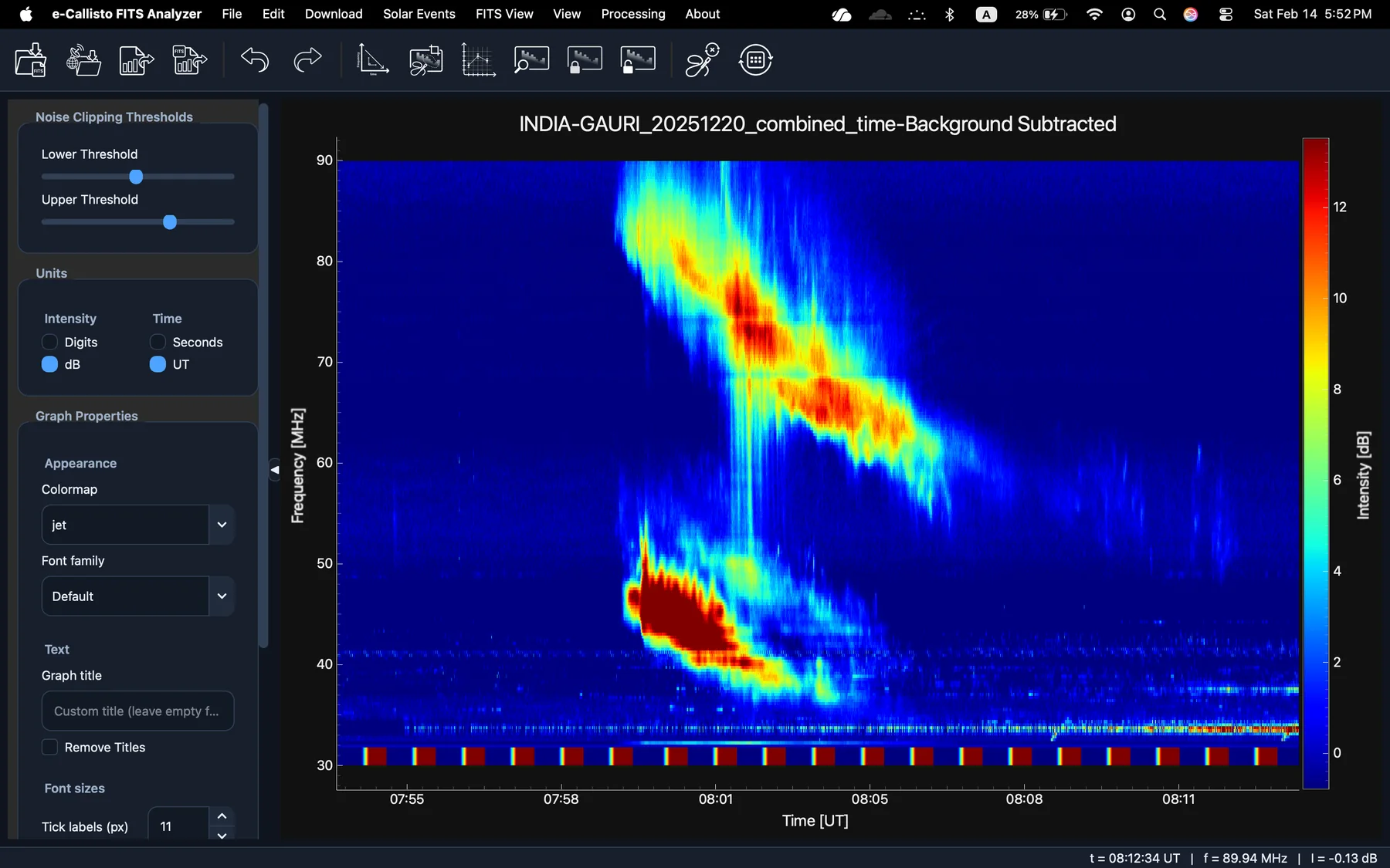
Reveal the signal
Inspect raw data before applying background subtraction. Adjust the display thresholds gradually. In v3.1.0, choose Mean, Median, or Median (dB), then Subtract Background.
Inspect the result
Look for coherent structure across time and frequency. Persistent horizontal features may be interference; compare raw and processed views before assigning a physical interpretation.
Keep your work
Save an .efaproj project. Export a figure and record the source filename and processing settings. You now have a traceable starting point for analysis.
Continue exploring
Consult the user guide for every control and method, or ask about your workflow in GitHub Discussions.